Feature selection
Every other module here builds one more feature. This one answers the question that follows: you have 200+ indicators — which of them are actually different from each other?
This module is not an expression API
selection is the deliberate exception to the expression
convention. Choosing
features is a cross-feature question that needs the whole materialized
matrix at once, so these functions take a pl.DataFrame and return NumPy
arrays and plain Python objects. Nothing here is on the .ta namespace,
and nothing here is lazy or streaming-safe.
Why you need this
polars_ta exposes over 200 indicators. They are nowhere near 200 independent
measurements: rsi(14), rsi(21), cmo, stochrsi and roc are one
underlying quantity read five ways. Handing all of them to a model is not just
wasteful — collinearity actively destroys feature-importance scores. Two
near-identical features split the credit between them and both look useless,
while a mediocre-but-unique third feature outranks them. This is the
substitution effect, and it breaks MDI and MDA alike.
So the order matters: remove redundancy first, score relevance second. This module is the first half. It never looks at a target, which is precisely why it is safe to run first — with no label involved, there is no label to leak.
Which features do I keep?
The short answer, and the one thing to take from this page:
result = selection.select_features(feats, FEATURES, k=6)
report = result.report()
report() gives one row per feature with a decision column. That column is
the answer.
decision |
Meaning | What to do |
|---|---|---|
keep |
This feature is its cluster's representative | Model on it |
drop |
Its representative correlates ≥ 0.7 with it | Discard — nothing is lost |
review |
Its representative correlates < 0.7 with it | Do not drop blindly — the partition is too coarse |
Real output, 16 indicators at k=4:
| feature | cluster | kept | representative | similarity | decision |
|---|---|---|---|---|---|
rsi_21 |
0 | ✅ | rsi_21 |
1.00 | keep |
rsi_14 |
0 | rsi_21 |
0.80 | drop | |
mfi |
0 | rsi_21 |
0.77 | drop | |
cmo_14 |
0 | rsi_21 |
0.75 | drop | |
roc_10 |
0 | rsi_21 |
0.66 | review | |
obv |
0 | rsi_21 |
0.62 | review | |
stochrsi |
1 | ✅ | stochrsi |
1.00 | keep |
adx_14 |
2 | ✅ | adx_14 |
1.00 | keep |
hurst |
2 | adx_14 |
0.76 | drop | |
vol_21 |
3 | ✅ | vol_21 |
1.00 | keep |
ulcer |
3 | vol_21 |
0.69 | review |
How to choose k: raise it until nothing says review
This is the concrete rule the rest of the page builds up to.
for k in (4, 6, 8):
    n = (select_features(feats, FEATURES, k=k).report()["decision"] == "review").sum()
    print(k, n)
# 4 → 4 flagged
# 6 → 0 flagged   ← use this
# 8 → 0 flagged
k=6 is the smallest cut where every drop is safe — and it agrees with
effective_rank (5.66), which is a reassuring independent check. Note that
signal_rank said 4, which was too aggressive: three features would have been
thrown away that nothing left behind could reconstruct.
Two numbers, one decision
effective_rank proposes k; the review count verifies it. If they
disagree, trust the review count — it is measured against the features
you actually have, not against a random-matrix assumption your data may
violate.
The pipeline
| Stage | Function | What it does |
|---|---|---|
| 0 | nonstationary_features |
Flag integrated features before you correlate anything |
| 0 | screen |
Materialize the matrix; drop sparse, warm-up and constant columns |
| 1 | corr_matrix |
Spearman (default) or Pearson correlation |
| 1 | vif |
Multicollinearity a pairwise screen cannot see |
| 1 | mutual_information |
Non-linear dependence; works on the sparse candle patterns |
| 1 | variation_of_information |
The same, as a true metric distance for clustering |
| 2 | denoise |
Marchenko-Pastur eigenvalue clipping, optional detoning |
| 3 | cluster_features |
Hierarchical clustering, k chosen by silhouette |
| 3 | cluster_by_distance |
The same engine on any distance — e.g. variation of information |
| 4 | select_representatives |
One feature per cluster |
| 1-4 | select_features |
Runs screen through select_representatives and returns a SelectionResult |
select_features deliberately does not run nonstationary_features for
you — fixing a flagged feature means choosing a transform, which is your call,
not a default. Run it first and act on what it reports.
Diagnostics: signal_rank and
effective_rank tell you how many
dimensions your feature set really has.
Stage 0 — stationarity is not optional
Correlations between integrated series are spurious (Granger & Newbold, 1974): two independent random walks correlate strongly by construction. Denoise a matrix built on raw levels and you are carefully denoising nonsense.
Several indicators in this library are integrated by design —
on_balance_volume, adi, volume_price_trend, cumulative_return, and every
price-level moving average. nonstationary_features flags them with a lag-1
autocorrelation screen (a heuristic, not a unit-root test). Fix a flagged
feature with quant.frac_diff — which keeps most of the memory —
or quant.rolling_z_score, then re-run.
Stage 2 — what Marchenko-Pastur actually tells you
For a correlation matrix built from \(T\) observations of \(N\) independent variables with variance \(\sigma^2\), the eigenvalues concentrate on
Any empirical eigenvalue below \(\lambda_+\) is therefore consistent with pure noise. With 205 features over 5000 bars, \(q \approx 24\) and \(\lambda_+ \approx 1.45\) — and the average eigenvalue of any correlation matrix is exactly 1, so that threshold cuts deep.
denoise replaces the entire noise bulk with its average. This preserves the
trace while destroying the spurious structure, and it lifts the smallest
eigenvalues away from zero — the practical payoff, since it is the
near-singular directions that wreck anything that inverts the matrix.
\(\sigma^2\) is estimated by fitting the theoretical MP density to a kernel density estimate of the observed eigenvalues (López de Prado, 2020, ch. 2). The tempting shortcut — iterate "everything below the edge is noise, its mean is the next \(\sigma^2\)" — is a trap: with real signal present it spirals downward until most of the bulk is misclassified as signal.
Detoning (detone=1) additionally strips the largest eigenvector. For
technical indicators on a single asset the dominant mode is essentially
"trend/level" and it swamps everything else, so detoning is what you want when
you are after features that say something beyond direction. It is off by
default because it is a modelling choice, not a correction.
Stage 3 — clustering, and why this distance
Unlike \(1 - \rho\), this is a true metric (Mantegna, 1999) — it satisfies the
triangle inequality, which is what makes hierarchical clustering on it
meaningful rather than merely suggestive. Note that perfectly anti-correlated
features land maximally far apart even though they carry the same information
with a flipped sign; pass np.abs(corr) if that matters for your feature set.
The number of clusters is chosen by maximising the mean silhouette (Rousseeuw, 1987) over every cut of the dendrogram — the correlation-clustering step of López de Prado's ONC, minus the recursive re-clustering of low-quality clusters.
Part 2 — is it real, and does it predict?
Everything above is target-free and therefore leak-free. These two are not, and they are where the answers get hard.
Significance: block_permute / permutation_test
With 200 candidate features, spurious winners are guaranteed. The defence is a
null distribution — but not from a plain shuffle, which would also destroy
the autocorrelation every rolling indicator has by construction and hand you a
null far too easy to beat. block_permute rebuilds each column from randomly
placed contiguous blocks of itself, so its serial dependence survives while its
alignment with every other column is destroyed.
This test found a real problem with signal_rank
Marchenko-Pastur assumes i.i.d. rows. Rolling indicators are ~0.99
autocorrelated, so n_obs grossly overstates the effective sample size and
the edge sits too low. On the 16-indicator case study:
| Statistic | Observed | Null | p |
|---|---|---|---|
| Eigenvalues above the edge | 4 | 5.1 ± 1.2 | 0.99 — not significant |
| Top eigenvalue | 6.07 | 1.54 ± 0.08 | 0.008 |
effective_rank |
5.66 | 15.5 | 0.008 |
The shared structure is unambiguously real; the precise count at the edge
is not. Prefer effective_rank as a headline, and treat signal_rank as a
ceiling unless you have tested it.
Relevance: the feature-importance toolkit
Everything above is target-free. This is the half that brings in a label — and therefore the half where leakage, the substitution effect and multiple testing all live at once.
Start with the cross-validation, because every measure below sits on top of it.
Purged K-fold with embargo (López de Prado, 2018, ch. 7) is not an
optimization, it is a correctness fix: bars \(t\) and \(t+1\) share \(w-1\)
observations of any \(w\)-window indicator, and a forward-return label spans \(h\)
more bars. A plain K-fold therefore trains on data that overlaps its own test
fold and reports memorization as skill. purged_kfold drops training samples
whose label window reaches into the test fold, then embargoes a further
\(h + \max(w)\) bars to handle the serial correlation in the features themselves.
| Function | Family | Looks at | Cost | Answers |
|---|---|---|---|---|
target_screen |
Filter | One feature at a time | Trivial | Does this co-move with the label at all? |
single_feature_importance |
Wrapper (SFI) | One cluster, alone | \(k\) fits/fold | What is this worth by itself? |
clustered_mdi |
Embedded (MDI) | All features, in-sample | Free with the fit | What did the model use? |
clustered_mda |
Wrapper (MDA) | All features, out-of-sample | \(k\) scores/fold | What breaks if I remove this last? |
clustered_shapley |
Wrapper | Every coalition | \(2^k\) fits/fold | What is this worth on average, over all orderings? |
null_importance |
Calibration | Any of the above | \(n_{\text{draws}} \times\) | Is any of it beyond chance? |
The model is always a callable you supply (fit/predict), so scikit-learn and
LightGBM stay your dependency, not this library's; RidgeRegressor is the
zero-dependency default. clustered_mdi is the one exception — it needs a model
that reports feature_importances_, so it has no default at all.
Step 1 — target_screen: the free triage
Before fitting anything, ask whether a feature moves with the label. Two statistics, both computed out of sample on the purged test folds:
- The information coefficient, a Spearman rank correlation (Grinold & Kahn, 1999). Rank rather than Pearson because one outlier bar otherwise sets the number. On real forward returns a mean \(|IC|\) of 0.02-0.05 is a useful feature; above 0.1 you should suspect your label before celebrating.
- Mutual information, which catches what an IC structurally cannot. A U-shaped relationship — both volatility tails predict, the middle does not — scores an IC of zero and an MI well above it. High MI with near-zero IC means non-monotone, not useless: it needs a model that can represent a fold.
ic_t_stat measures consistency, not size
A negligible-but-reliably-signed IC gets a large t-stat. In this library's
own tests a pure-noise feature scores \(|IC|\) 0.008 with a t-stat near 5 —
a stable nothing. Sort by abs_ic; use the t-stat only to discard what
near the top fails to reproduce across folds.
Step 2 — the three classical measures, and why you run all three
MDI, MDA and SFI (López de Prado, 2018 ch. 8; 2020 ch. 6) are not competing implementations of one idea. They answer three different questions, and their disagreement is the diagnostic:
- MDI — in-sample impurity reduction, summed within each cluster. Free with a tree fit and the only measure that sees interactions directly, since a deep split is conditional on everything above it. But it is in-sample, it is biased toward high-cardinality features (a continuous feature offers a tree far more split points than a 0/±100 candlestick pattern), and it has no null — a pure-noise feature still scores above zero.
- MDA — the drop in out-of-sample score when a cluster is shuffled. The strongest of the three, and the only one with a natural zero.
- SFI — fit each cluster alone. Structurally immune to substitution because nothing is left to substitute with, and equally blind to interaction.
| SFI | MDA | Reading |
|---|---|---|
| high | high | Genuinely predictive. Keep. |
| high | low | Redundant — something else already carries it. |
| low | high | Only works in combination. Keep, but never alone. |
| low | low | Nothing there. |
Similarly, high MDI with zero MDA means the model memorized that feature — the single most useful cross-check the pair provides.
Step 3 — clustered_shapley: the one that adds up
MDA asks what breaks if a cluster is removed last; SFI asks what it earns first. On interacting features those differ, with no principled reconciliation — which is exactly what the Shapley value provides, by averaging a cluster's marginal contribution over every order in which clusters could be added:
SFI is the \(S = \emptyset\) term, MDA is close to the \(S = N \setminus \{i\}\) term, and \(\phi_i\) is the properly weighted average of those and everything between. The payoff is efficiency: the values sum exactly to the full model's score over an empty one, so "cluster 0 is 40% of the edge" becomes a defensible statement rather than a vibe. It is also the only measure here that reports a negative importance honestly.
Cost is \(2^k\) fits per fold
32 fits for \(k=5\), 4096 for \(k=12\), times n_splits. This is why the
function takes clusters rather than features — per-feature Shapley on a
200-column matrix is not slow, it is infeasible. max_clusters (default 12)
exists to stop you finding that out the hard way.
Step 4 — null_importance: the number that decides
An importance of 0.03 is not a finding until you know what 0.03 looks like when nothing is there — and it is rarely zero. With 200 candidates, a flexible model and a weak label, the best cluster always shows a positive score.
The fix (Altmann et al., 2010) breaks the one link that matters — feature to
label — and leaves everything else intact. Features keep their correlation
structure, the model keeps its capacity, the CV keeps its geometry; only the
target is scrambled, and it is scrambled with block_permute rather than a
plain shuffle, because a forward return is autocorrelated and destroying that
too would make the null far too easy to beat.
null = selection.null_importance(
    scored, sel.names, "fwd", labels=sel.labels,
    n_draws=100, label_horizon=12, embargo=300,
)
null.report()                  # observed vs chance, with z-scores
null.significant(alpha=0.05)   # the ids surviving Bonferroni
significant() applies a Bonferroni correction by default, because testing
20 clusters at \(\alpha = 0.05\) produces a false positive about 64% of the time.
Note that n_draws floors the smallest resolvable p-value at
\(1/(n_\text{draws}+1)\) — 50 draws cannot resolve below 0.02, which is not enough
to clear Bonferroni past a handful of clusters.
Worked example: the whole library against a real label
examples/plot_feature_importance.py runs all six on every indicator
polars_ta exposes — 205 built automatically, screened to 183 — clustered
into 8 groups and ranked against a 12-bar forward return on 5000 BTCUSDT 5m
bars, with label_horizon=12 and embargo=300.
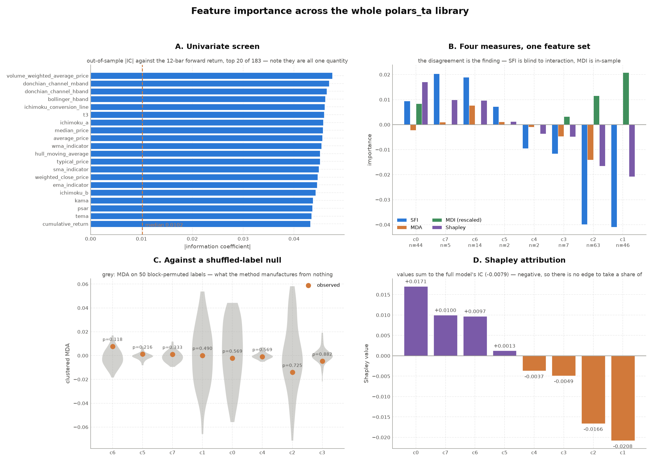
The univariate screen looks encouraging at first: the top features reach
\(|IC| \approx 0.047\) with t-stats near 3.8, which on a research desk would pass
for a signal. Then the model-based measures arrive — MDI from a
RandomForestRegressor (120 trees, depth 4), the rest from the default ridge:
| Cluster | n | Example member | SFI | MDA | MDI | Shapley |
|---|---|---|---|---|---|---|
| 0 | 44 | acc_dist_index |
0.0095 | −0.0022 | 0.191 | 0.0171 |
| 7 | 5 | cdl_harami |
0.0203 | 0.0010 | 0.000 | 0.0100 |
| 6 | 14 | cdl_3_white_soldiers |
0.0190 | 0.0077 | 0.001 | 0.0097 |
| 5 | 2 | cdl_3_line_strike |
0.0073 | 0.0012 | 0.000 | 0.0013 |
| 4 | 2 | cdl_2_crows |
−0.0095 | −0.0009 | 0.003 | −0.0037 |
| 3 | 7 | approximate_entropy |
−0.0116 | −0.0047 | 0.074 | −0.0049 |
| 2 | 63 | adx_pos |
−0.0399 | −0.0141 | 0.262 | −0.0166 |
| 1 | 46 | adx |
−0.0409 | 0.0001 | 0.469 | −0.0208 |
The full-model out-of-sample IC is −0.0079. Negative. The Shapley values sum to exactly that, as efficiency requires.
MDI ranks the ranking exactly backwards
This is the memorization signature, on real data. The forest spends 47% of its total impurity reduction on cluster 1 — more than on all seven other clusters' worth of continuous features combined — and that cluster's out-of-sample MDA is 0.0001, its Shapley value −0.021. Clusters 1 and 2 together take 73% of the MDI budget while contributing nothing out of sample.
Meanwhile the three candlestick clusters (5, 6, 7) score essentially zero
MDI — 0.001 between them — despite cluster 6 having the best MDA and the
lowest p-value of any cluster in the study. That is MDI's cardinality bias
stated in numbers: a continuous feature offers a tree hundreds of split
points, a 0/±100 pattern offers two, and MDI rewards the former for the
opportunity alone.
Read MDI alone and you would keep the 109 trend/momentum features and throw away the only cluster that came close to significance.
Not one cluster survives the null
With 50 shuffled-label draws, the best p-value is 0.118 (cluster 6) and nothing clears Bonferroni at 5% — or even an uncorrected 5%. The encouraging \(|IC| = 0.047\) from the univariate screen does not survive contact with a model, purged cross-validation, and a null.
This is the correct result, not a failed experiment. 200 technical indicators on 5000 bars of one asset, against a 12-bar forward return, do not predict it. A pipeline that reported otherwise would be measuring its own leakage. Every guard in this module — purging, embargoing, block permutation, Bonferroni — exists to make this the outcome rather than a confident, wrong number.
Two secondary readings worth taking from the same table:
- SFI and MDA disagree sharply on clusters 1 and 2 (SFI ≈ −0.04, MDA ≈ 0). Read via the table above, that is the low-SFI / low-MDA quadrant with noise on top: these 109 trend and momentum features are worthless alone and cost nothing when removed.
- Cluster 0 has the top Shapley value but a negative MDA. Its contribution is real only in combination, and only in some orderings — the precise case MDA alone would have scored as harmful and SFI alone as mediocre. It is also well within the null, so the honest conclusion is still "nothing here".
Feature selection: find the handful of independent signals hiding in a wide indicator matrix.
Every other module in this library produces a pl.Expr — one column, computed
lazily. This module is the exception, and deliberately so: choosing features is
a cross-feature question that needs the whole materialized matrix at once, so
these functions take a pl.DataFrame and return NumPy arrays and plain Python
containers. Nothing here is registered on the .ta namespace.
The problem it solves: polars_ta exposes 200+ indicators, and they are
nowhere near 200 independent measurements. rsi(14), rsi(21), cmo,
stochrsi and roc are one underlying quantity read five ways. Feeding all of
them to a model is not just wasteful — collinearity actively destroys every
per-feature importance score, because two near-identical features split the
credit between them and both look useless (the "substitution effect").
So the work splits in two, and the order is not negotiable.
Part 1 — redundancy (no target, therefore no possible leakage):
screen— materialize the matrix, drop sparse, warm-up and degenerate columns.corr_matrix/mutual_information/vif— linear, rank, and non-linear dependence, plus multicollinearity that pairwise screening misses.denoise— Marchenko-Pastur eigenvalue clipping: everything below the random-matrix edge is indistinguishable from noise, so it is flattened rather than trusted. Optionally detone the dominant market mode.cluster_features/cluster_by_distance— hierarchical clustering on the correlation distance or on variation of information.select_representatives— one feature per cluster.
select_features runs 1-5 and hands back a SelectionResult. Run
nonstationary_features yourself first — correlations between integrated
series are spurious, and select_features does not apply a fix for you
because choosing the transform is a modelling decision, not a default.
Part 2 — is it real, and does it predict?
permutation_testwithblock_permute— a null distribution for any statistic of the matrix. With 200 candidate features, spurious winners are guaranteed; this is what distinguishes structure from chance.target_screen— the cheap univariate triage: information coefficient and mutual information against the label, per feature, out of sample. No model, so no model to blame; run it before anything expensive.clustered_mdawithpurged_kfold— importance against an actual target. This does look at a label, so it is where leakage lives: the cross-validation purges and embargoes overlapping samples, and shuffling is done per cluster so the substitution effect cannot scramble the scores.clustered_mdi— the in-sample counterpart, for tree models that reportfeature_importances_. Fast and free with the fit, but in-sample and biased toward high-cardinality features, so it is a cross-check on MDA, not a replacement.single_feature_importance(SFI) — fit each feature alone. Structurally immune to substitution (nothing is left to substitute with) and equally blind to interaction, which makes the MDA/MDI/SFI disagreement itself informative.clustered_shapley— exact Shapley attribution of the out-of-sample score across clusters. Unlike MDA it is additive: the values sum to what the full model earns over an empty one, so "cluster A is worth 40% of the edge" is a statement you can actually make.null_importance— refit against a shuffled label many times to get a per-cluster null. This turns any of the scores above into a p-value, which is the only defensible way to draw the keep/drop line on 200 candidates.
The three importance families answer different questions and are meant to be read together (López de Prado, 2020, ch. 6): MDI says what the model used in-sample, MDA what it needs out of sample, SFI what each feature is worth alone. A feature that scores high on MDI and zero on MDA was memorized; high on SFI and zero on MDA is redundant with something else; high on MDA and low on SFI only works in combination.
References
- Marchenko & Pastur (1967), Distribution of eigenvalues for some sets of random matrices.
- López de Prado (2018), Advances in Financial Machine Learning, ch. 7 (purged K-fold cross-validation with embargo) and ch. 8 (MDI, MDA and SFI feature importance).
- López de Prado (2020), Machine Learning for Asset Managers, ch. 2 (denoising and detoning), ch. 3 (information-theoretic distance), ch. 4 (optimal clustering) and ch. 6 (clustered MDI and MDA).
- Mantegna (1999), Hierarchical structure in financial markets — the correlation-to-distance metric.
- Meila (2007), Comparing clusterings — variation of information as a metric.
- Rousseeuw (1987), Silhouettes — choosing the number of clusters.
- Hacine-Gharbi et al. (2012) — optimal histogram binning for mutual information.
- Altmann et al. (2010), Permutation importance: a corrected feature
importance measure — the shuffled-label null behind
null_importance. - Shapley (1953), A value for n-person games; Štrumbelj & Kononenko (2014) for its use as a feature attribution.
- Grinold & Kahn (1999), Active Portfolio Management — the information coefficient as the unit of predictive skill.
dataclass

ScreenResult(values: ndarray, names: list[str], dropped: list[str] = list(), n_rows_dropped: int = 0, sparse: list[str] = list(), missing_rate: dict[str, float] = dict())
Output of :func:screen — a clean feature matrix and what was removed.
worst_missing(limit: int = 5) -> list[tuple[str, float]]
The limit columns with the highest non-finite rate, worst first.
Reach for this when n_rows_dropped is large: row removal is driven by
the worst column, so a single sparse feature can cost the whole
matrix most of its sample.
Source code in polars_ta/selection.py
169 170 171 172 173 174 175 176 177 | |
dataclass

SelectionResult(selected: list[str], clusters: dict[int, list[str]], labels: ndarray, names: list[str], dropped: list[str], corr: ndarray, silhouette: float, signal_rank: int, effective_rank: float, n_obs: int)
Output of :func:select_features.
report(min_similarity: float = 0.7) -> DataFrame
Per-feature keep/drop table, with the evidence for each decision.
selected tells you what survived; this tells you why, and — more
usefully — which of the drops you should not trust.
A cluster representative stands in for its members only as well as it
correlates with them. Dropping a feature that correlates 0.97 with the
kept one costs you nothing; dropping one that correlates 0.35 throws
away real information, and means the partition was too coarse. Those
two cases are indistinguishable in selected alone, which is why this
exists.
Columns:
| Column | Meaning |
|---|---|
feature |
The feature name |
cluster |
Which cluster it landed in |
cluster_size |
How many features share that cluster |
kept |
Whether it is the cluster's representative |
representative |
The feature kept in its place |
similarity |
abs correlation to that representative, in [0, 1] |
decision |
"keep", "drop", or "review" |
The decision rule:
keep— this is the representative; model on it.drop—similarity >= min_similarity, so the representative carries what this feature carried. Safe to discard.review—similarity < min_similarity. The representative is a poor stand-in. Either raisekso this feature gets its own cluster, or keep it alongside the representative.
A high review count means the clustering was cut too coarse, and is
the signal to increase k — a more grounded way to choose it than
silhouette alone.
report = result.report()
report.filter(pl.col("decision") == "review")   # the risky drops
report.filter(pl.col("kept"))                   # the final feature set
Note that similarity uses absolute correlation: a representative
correlating -0.95 with a member carries that member's information with
a flipped sign, which a linear model recovers for free.
Parameters:
| Name | Type | Description | Default |
|---|---|---|---|
min_similarity
|
float
|
Correlation below which a drop is flagged for review rather than treated as safe. |
0.7
|
Returns:
| Type | Description |
|---|---|
DataFrame
|
One row per surviving feature, sorted by cluster then by descending |
DataFrame
|
similarity, so each cluster reads as "the kept one, then what it |
DataFrame
|
replaced, worst last". |
Source code in polars_ta/selection.py
205 206 207 208 209 210 211 212 213 214 215 216 217 218 219 220 221 222 223 224 225 226 227 228 229 230 231 232 233 234 235 236 237 238 239 240 241 242 243 244 245 246 247 248 249 250 251 252 253 254 255 256 257 258 259 260 261 262 263 264 265 266 267 268 269 270 271 272 273 274 275 276 277 278 279 280 281 282 283 284 285 286 287 288 289 290 291 292 293 | |
dataclass

PermutationTest(observed: float, null: ndarray, p_value: float, alternative: str)
RidgeRegressor(alpha: float = 1.0)
A minimal ridge regression, used as :func:clustered_mda's default model.
Exists so importance scoring works out of the box without pulling scikit-learn
into a library whose dependencies are Polars and NumPy. It is deliberately
plain — swap in any object exposing fit(X, y) and predict(X) (an sklearn
estimator, a gradient-boosted tree) via model_factory when you want
something with more capacity.
Ridge rather than ordinary least squares because a feature matrix drawn from this library is routinely singular to machine precision, where OLS has no unique solution at all.
Source code in polars_ta/selection.py
1467 1468 1469 1470 | |
fit(x: ndarray, y: ndarray) -> RidgeRegressor
Fit on centered data, keeping the intercept out of the penalty.
Source code in polars_ta/selection.py
1472 1473 1474 1475 1476 1477 1478 1479 1480 | |
predict(x: ndarray) -> ndarray
Predict for x.
Source code in polars_ta/selection.py
1482 1483 1484 | |
dataclass

ImportanceResult(clusters: dict[int, list[str]], importance: dict[int, float], std: dict[int, float], baseline: float, n_splits: int)
Output of the clustered importance routines.
Returned by :func:clustered_mda, :func:clustered_mdi,
:func:single_feature_importance and :func:clustered_shapley, so the four
are directly comparable — same keys, same ordering, same ranked property.
What the number means differs by routine (a score drop for MDA and
Shapley, an impurity share for MDI, a standalone score for SFI), which is
why they should be compared by rank rather than by level.
t_stats() -> dict[int, float]
Per-cluster mean / (std / sqrt(n_splits)).
A crude significance check across folds. An importance whose sign is not stable fold-to-fold is not an importance — and with few folds this statistic is itself noisy, so read it as a smell test, not a p-value.
Source code in polars_ta/selection.py
1575 1576 1577 1578 1579 1580 1581 1582 1583 1584 1585 1586 1587 1588 | |
dataclass

NullImportanceResult(clusters: dict[int, list[str]], observed: dict[int, float], null: dict[int, ndarray], p_value: dict[int, float])
Output of :func:null_importance.
significant(alpha: float = 0.05, correction: str = 'bonferroni') -> set[int]
Cluster ids whose importance beats the null at level alpha.
Parameters:
| Name | Type | Description | Default |
|---|---|---|---|
alpha
|
float
|
Family-wise error rate to control. |
0.05
|
correction
|
str
|
|
'bonferroni'
|
Returns:
| Type | Description |
|---|---|
set[int]
|
The surviving cluster ids. |
Raises:
| Type | Description |
|---|---|
ValueError
|
If |
Source code in polars_ta/selection.py
2231 2232 2233 2234 2235 2236 2237 2238 2239 2240 2241 2242 2243 2244 2245 2246 2247 2248 2249 2250 2251 2252 2253 2254 2255 2256 2257 | |
report() -> DataFrame
Per-cluster table: observed importance, null mean, z-score, p-value.
Columns are cluster, features, observed, null_mean, null_std,
z_score and p_value, sorted by ascending p-value. The z_score is
(observed - null_mean) / null_std — how many null standard deviations
the real importance sits above chance, which stays informative when the
p-value floors at 1/(n_draws+1).
Source code in polars_ta/selection.py
2259 2260 2261 2262 2263 2264 2265 2266 2267 2268 2269 2270 2271 2272 2273 2274 2275 2276 2277 2278 2279 2280 2281 2282 2283 2284 2285 2286 2287 | |
screen(df: DataFrame, features: Sequence[str] | None = None, max_missing: float | None = None) -> ScreenResult
Turn a frame of indicator columns into a clean, finite feature matrix.
Three kinds of garbage are removed, all of which silently corrupt a correlation matrix if left in:
- Sparse columns (opt-in, via
max_missing). Row removal is driven by the worst column, so one feature that is frequently undefined costs every other feature its sample. This is not hypothetical: on the full indicator library,roll_spreadis null wherever its serial-covariance premise fails — about 42% of bars, scattered throughout — and on its own it takes a 5,000-bar sample down to 2,610 rows for all 184 features. Settingmax_missing=0.2drops such a column instead of letting it truncate the matrix.worst_missing()on the result names the culprits. - Warm-up rows. Indicators have wildly different warm-up lengths (an
EMA(9) is live after 9 bars,
momentum_12_1after 273). Any row where any surviving feature is null, NaN or infinite is dropped, so every pairwise correlation is computed on the same aligned sample. - Constant columns. A zero-variance feature has undefined correlation
and puts
NaNinto the matrix, which then poisons the entire eigendecomposition. Also not hypothetical: on a 5,000-bar sample, 21 of the 61 candlestick patterns never fire even once.
Parameters:
| Name | Type | Description | Default |
|---|---|---|---|
df
|
DataFrame
|
Frame containing the feature columns. |
required |
features
|
Sequence[str] | None
|
Column names to use. Defaults to every numeric column. |
None
|
max_missing
|
float | None
|
Drop any column whose non-finite fraction exceeds this,
before dropping rows. |
None
|
Returns:
| Name | Type | Description |
|---|---|---|
A |
ScreenResult
|
class: |
Raises:
| Type | Description |
|---|---|
ValueError
|
If a requested column is missing or non-numeric, if
|
Source code in polars_ta/selection.py
301 302 303 304 305 306 307 308 309 310 311 312 313 314 315 316 317 318 319 320 321 322 323 324 325 326 327 328 329 330 331 332 333 334 335 336 337 338 339 340 341 342 343 344 345 346 347 348 349 350 351 352 353 354 355 356 357 358 359 360 361 362 363 364 365 366 367 368 369 370 371 372 373 374 375 376 377 378 379 380 381 382 383 384 385 386 387 388 389 390 391 392 393 394 395 396 397 398 399 400 401 402 403 404 405 | |
nonstationary_features(df: DataFrame, features: Sequence[str] | None = None, threshold: float = 0.99) -> list[str]
Flag features whose level behaves like an integrated series.
Correlations between non-stationary series are spurious (Granger & Newbold,
1974) — two independent random walks correlate strongly by construction —
so running the rest of this module on raw levels denoises nonsense. Several
indicators in this library are integrated by design: on_balance_volume,
adi, volume_price_trend, cumulative_return, and every price-level
moving average.
The screen is a cheap heuristic, not a unit-root test: lag-1
autocorrelation of the level. A near-unit value means the series barely
mean-reverts bar to bar. Fix a flagged feature with
:func:polars_ta.quant.frac_diff (keeps most of the memory) or
:func:polars_ta.quant.rolling_z_score, then re-run.
Parameters:
| Name | Type | Description | Default |
|---|---|---|---|
df
|
DataFrame
|
Frame containing the feature columns. |
required |
features
|
Sequence[str] | None
|
Column names to test. Defaults to every numeric column. |
None
|
threshold
|
float
|
Lag-1 autocorrelation at or above which a feature is flagged. |
0.99
|
Returns:
| Type | Description |
|---|---|
list[str]
|
The flagged column names, in input order. Columns that are constant (so |
list[str]
|
autocorrelation is undefined) are not flagged — :func: |
list[str]
|
those separately. |
Source code in polars_ta/selection.py
408 409 410 411 412 413 414 415 416 417 418 419 420 421 422 423 424 425 426 427 428 429 430 431 432 433 434 435 436 437 438 439 440 441 442 443 444 445 446 447 448 449 450 | |
corr_matrix(values: ndarray, method: str = 'spearman') -> ndarray
Correlation matrix of a (n_obs, n_features) matrix.
Parameters:
| Name | Type | Description | Default |
|---|---|---|---|
values
|
ndarray
|
Finite feature matrix, e.g. |
required |
method
|
str
|
|
'spearman'
|
Returns:
| Type | Description |
|---|---|
ndarray
|
A symmetric |
Raises:
| Type | Description |
|---|---|
ValueError
|
If |
Source code in polars_ta/selection.py
466 467 468 469 470 471 472 473 474 475 476 477 478 479 480 481 482 483 484 485 486 487 488 489 490 491 492 | |
vif(corr: ndarray, ridge: float = 1e-10) -> ndarray
Variance inflation factor per feature.
\(\mathrm{VIF}_i = 1/(1 - R_i^2)\), where \(R_i^2\) is from regressing feature
\(i\) on all the others — equivalently the \(i\)-th diagonal entry of the
inverted correlation matrix. It answers a different question from a
pairwise correlation: a feature can correlate weakly with every other
feature individually and still be an exact linear combination of several
of them, which pairwise screening never sees. macd versus a pair of EMAs
is exactly that case.
Conventional reading: VIF > 5 is worth a look, > 10 is severe. On a wide indicator matrix expect values in the thousands — which is the finding, not a bug.
Computed by eigendecomposition as
\(\mathrm{VIF}_i = \sum_j V_{ij}^2 / (\lambda_j + \varepsilon)\) rather than
by inverting the matrix. A wide indicator matrix is routinely singular to
machine precision (the full library reaches a condition number of ~1e21),
where inv returns noise and — worse — pinv quietly hides the problem:
the pseudo-inverse discards the null space, so exactly-collinear features
come back with a reassuring VIF of 1.0. The ridge keeps the blow-up
visible and finite instead.
Parameters:
| Name | Type | Description | Default |
|---|---|---|---|
corr
|
ndarray
|
Symmetric correlation matrix with a unit diagonal. |
required |
ridge
|
float
|
Added to each eigenvalue before inversion. Sets the ceiling on
a reported VIF (roughly |
1e-10
|
Returns:
| Type | Description |
|---|---|
ndarray
|
One VIF per feature, aligned with |
Source code in polars_ta/selection.py
495 496 497 498 499 500 501 502 503 504 505 506 507 508 509 510 511 512 513 514 515 516 517 518 519 520 521 522 523 524 525 526 527 528 529 530 531 | |
mutual_information(values: ndarray, bins: int | None = None, normalize: bool = True) -> ndarray
Pairwise mutual information matrix.
\(I(X;Y) = H(X) + H(Y) - H(X,Y)\), estimated from a 2-D histogram. Unlike correlation it is not limited to monotone association, and it handles the sparse discrete features (candlestick patterns) that make a rank correlation near-useless.
Parameters:
| Name | Type | Description | Default |
|---|---|---|---|
values
|
ndarray
|
Finite |
required |
bins
|
int | None
|
Histogram bins per axis. Defaults to the Hacine-Gharbi optimum for the sample size. |
None
|
normalize
|
bool
|
Divide by |
True
|
Returns:
| Type | Description |
|---|---|
ndarray
|
A symmetric |
ndarray
|
normalized (a feature determines itself), else its own entropy. |
Source code in polars_ta/selection.py
572 573 574 575 576 577 578 579 580 581 582 583 584 585 586 587 588 589 590 591 592 593 594 595 596 597 598 599 600 601 602 603 604 605 606 607 608 609 610 611 | |
variation_of_information(values: ndarray, bins: int | None = None) -> ndarray
Normalized variation of information — a metric distance.
\(VI(X;Y) = H(X,Y) - I(X;Y)\), divided by \(H(X,Y)\) to land in \([0, 1]\). It
satisfies the triangle inequality (Meila, 2007), which is what makes it a
legitimate input to :func:cluster_by_distance — and it is the non-linear
counterpart to :func:distance_matrix: 0 when two features determine each
other, 1 when they are independent.
Use it instead of the correlation distance when the feature set contains discrete or sparse columns, or when you suspect non-monotone relationships that Spearman scores as zero.
Parameters:
| Name | Type | Description | Default |
|---|---|---|---|
values
|
ndarray
|
Finite |
required |
bins
|
int | None
|
Histogram bins per axis; defaults to the Hacine-Gharbi optimum. |
None
|
Returns:
| Type | Description |
|---|---|
ndarray
|
A symmetric distance matrix with a zero diagonal. |
Source code in polars_ta/selection.py
614 615 616 617 618 619 620 621 622 623 624 625 626 627 628 629 630 631 632 633 634 635 636 637 638 639 640 641 642 643 644 645 646 647 | |
marcenko_pastur_edge(q: float, sigma2: float = 1.0) -> float
Upper edge of the Marchenko-Pastur eigenvalue support.
For a correlation matrix built from n_obs observations of n_features
independent variables with variance \(\sigma^2\), the eigenvalues
concentrate on \([\lambda_-, \lambda_+]\) with
Any empirical eigenvalue below \(\lambda_+\) is therefore consistent with pure noise. With 205 features over 5000 bars, \(q \approx 24\) and \(\lambda_+ \approx 1.45\) — a sobering threshold, since the average eigenvalue of any correlation matrix is exactly 1.
Parameters:
| Name | Type | Description | Default |
|---|---|---|---|
q
|
float
|
Aspect ratio |
required |
sigma2
|
float
|
Noise variance. |
1.0
|
Returns:
| Type | Description |
|---|---|
float
|
The upper edge \(\lambda_+\). |
Raises:
| Type | Description |
|---|---|
ValueError
|
If |
Source code in polars_ta/selection.py
655 656 657 658 659 660 661 662 663 664 665 666 667 668 669 670 671 672 673 674 675 676 677 678 679 680 681 682 683 684 685 | |
denoise(corr: ndarray, q: float, detone: int = 0, bandwidth: float = 0.01) -> ndarray
Marchenko-Pastur denoising of a correlation matrix.
Eigenvalues below the MP edge carry no information beyond what a matrix of independent noise would produce, but they are the smallest ones — so anything that inverts or optimizes over the raw matrix is dominated by them. Clipping replaces the whole noise bulk with its average, which kills the spurious structure while preserving the trace (and therefore the unit diagonal, up to the rescaling applied at the end).
Parameters:
| Name | Type | Description | Default |
|---|---|---|---|
corr
|
ndarray
|
Symmetric correlation matrix with a unit diagonal. |
required |
q
|
float
|
Aspect ratio |
required |
detone
|
int
|
Number of leading (largest) eigenvalues to remove entirely.
|
0
|
bandwidth
|
float
|
Kernel bandwidth for the eigenvalue density fit that estimates the noise variance. The default suits the hundreds of eigenvalues a wide indicator matrix produces; widen it for a narrow matrix, where the empirical density is spiky. |
0.01
|
Returns:
| Type | Description |
|---|---|
ndarray
|
The denoised correlation matrix, symmetric with a unit diagonal. |
Raises:
| Type | Description |
|---|---|
ValueError
|
If |
Source code in polars_ta/selection.py
774 775 776 777 778 779 780 781 782 783 784 785 786 787 788 789 790 791 792 793 794 795 796 797 798 799 800 801 802 803 804 805 806 807 808 809 810 811 812 813 814 815 816 817 818 819 820 821 822 823 824 825 826 827 828 829 830 | |
signal_rank(corr: ndarray, q: float, bandwidth: float = 0.01) -> int
Number of eigenvalues above the Marchenko-Pastur edge.
A first answer to "how many features do I actually have?". For a matrix of pure independent noise this is 0; for 205 technical indicators on one asset, expect somewhere in the teens.
Read this as a ceiling, not a measurement
The Marchenko-Pastur law assumes i.i.d. rows, and rolling
indicators violate that badly — a 14-period ATR has lag-1
autocorrelation around 0.997, so n_obs wildly overstates the
effective sample size and the edge lands too low.
Measured on the BTCUSDT 5m fixture with 16 indicators: the observed
count is 4, but a :func:block_permute null that keeps each feature's
autocorrelation and destroys only the cross-feature alignment produces
5.1 ± 1.0 — so the count itself is not distinguishable from chance
(p ≈ 1.0). The same null leaves the top eigenvalue (6.07 vs 1.54) and
:func:effective_rank (5.66 vs 15.5) overwhelmingly significant.
In other words: the existence of strong shared structure is real, and
the eigenvalues far above the edge are real. The precise count of those
hovering at it is not. Use :func:permutation_test to find out which
regime you are in rather than trusting this number on its own, and
prefer :func:effective_rank as the headline figure.
Parameters:
| Name | Type | Description | Default |
|---|---|---|---|
corr
|
ndarray
|
Symmetric correlation matrix with a unit diagonal. |
required |
q
|
float
|
Aspect ratio |
required |
bandwidth
|
float
|
Kernel bandwidth for the noise-variance fit; see
:func: |
0.01
|
Returns:
| Type | Description |
|---|---|
int
|
The count of eigenvalues strictly above the estimated edge. |
Source code in polars_ta/selection.py
833 834 835 836 837 838 839 840 841 842 843 844 845 846 847 848 849 850 851 852 853 854 855 856 857 858 859 860 861 862 863 864 865 866 867 868 869 870 871 | |
effective_rank(corr: ndarray) -> float
Entropy-based effective rank (Roy & Vetterli, 2007).
\(\exp(H)\) where \(H = -\sum_i p_i \ln p_i\) and
\(p_i = \lambda_i / \sum_j \lambda_j\). A continuous companion to
:func:signal_rank that needs no noise model: it is n_features when the
features are perfectly independent and 1 when they are perfectly
collinear, so the ratio to n_features reads directly as "fraction of the
matrix that is genuinely distinct".
Parameters:
| Name | Type | Description | Default |
|---|---|---|---|
corr
|
ndarray
|
Symmetric correlation matrix with a unit diagonal. |
required |
Returns:
| Type | Description |
|---|---|
float
|
The effective rank, in |
Source code in polars_ta/selection.py
874 875 876 877 878 879 880 881 882 883 884 885 886 887 888 889 890 891 892 893 894 | |
distance_matrix(corr: ndarray) -> ndarray
Correlation-to-distance metric \(d_{ij} = \sqrt{(1-\rho_{ij})/2}\).
Unlike \(1-\rho\), this is a true metric (Mantegna, 1999) — it satisfies the triangle inequality, which is what makes hierarchical clustering on it meaningful rather than merely suggestive. It maps \(\rho = 1\) to 0, \(\rho = 0\) to \(1/\sqrt{2}\), and \(\rho = -1\) to 1.
Note that perfectly anti-correlated features land far apart, even though
they carry the same information with a flipped sign. If that matters for
your feature set, pass np.abs(corr) in.
Parameters:
| Name | Type | Description | Default |
|---|---|---|---|
corr
|
ndarray
|
Symmetric correlation matrix with a unit diagonal. |
required |
Returns:
| Type | Description |
|---|---|
ndarray
|
A symmetric distance matrix with a zero diagonal. |
Source code in polars_ta/selection.py
902 903 904 905 906 907 908 909 910 911 912 913 914 915 916 917 918 919 920 921 922 923 924 | |
silhouette_score(dist: ndarray, labels: ndarray) -> float
Mean silhouette of a partition (Rousseeuw, 1987).
For each feature, a is its mean distance to its own cluster and b its
mean distance to the nearest other cluster; the silhouette is
(b - a) / max(a, b). Near 1 means the clusters are tight and
well-separated, near 0 means they overlap, negative means features are
closer to a neighbouring cluster than their own.
Members of singleton clusters score 0, the usual convention — a lone feature is neither well nor badly placed.
Parameters:
| Name | Type | Description | Default |
|---|---|---|---|
dist
|
ndarray
|
Symmetric distance matrix. |
required |
labels
|
ndarray
|
Cluster id per feature. |
required |
Returns:
| Type | Description |
|---|---|
float
|
The mean silhouette, in |
float
|
partition (one cluster, or every feature in its own). |
Source code in polars_ta/selection.py
967 968 969 970 971 972 973 974 975 976 977 978 979 980 981 982 983 984 985 986 987 988 989 990 991 992 993 994 995 996 997 998 999 1000 1001 1002 1003 1004 | |
cluster_features(corr: ndarray, max_k: int | None = None, k: int | None = None) -> tuple[ndarray, float]
Cluster features by correlation distance, picking k by silhouette.
Average-linkage agglomerative clustering on
:func:distance_matrix, cut at every k from 2 to max_k and scored by
:func:silhouette_score; the best-scoring cut wins. This is the
correlation-clustering step of López de Prado's ONC, minus the recursive
re-clustering of low-quality clusters.
Parameters:
| Name | Type | Description | Default |
|---|---|---|---|
corr
|
ndarray
|
Symmetric correlation matrix with a unit diagonal — denoise it first, otherwise you are clustering on noise. |
required |
max_k
|
int | None
|
Largest number of clusters to consider. Defaults to
|
None
|
k
|
int | None
|
Force an exact number of clusters instead of choosing by silhouette.
The natural argument is :func: |
None
|
Returns:
| Type | Description |
|---|---|
ndarray
|
|
float
|
silhouette of the chosen partition. |
Raises:
| Type | Description |
|---|---|
ValueError
|
If there are fewer than 3 features, if |
Source code in polars_ta/selection.py
1007 1008 1009 1010 1011 1012 1013 1014 1015 1016 1017 1018 1019 1020 1021 1022 1023 1024 1025 1026 1027 1028 1029 1030 1031 1032 1033 1034 1035 1036 1037 | |
cluster_by_distance(dist: ndarray, max_k: int | None = None, k: int | None = None) -> tuple[ndarray, float]
Cluster on any feature distance matrix.
The engine behind :func:cluster_features, exposed separately so the
distance need not come from a correlation. Pass
:func:variation_of_information to cluster on non-linear dependence
instead — the right choice when the feature set includes the sparse,
discrete candlestick patterns, which a rank correlation barely sees.
Parameters:
| Name | Type | Description | Default |
|---|---|---|---|
dist
|
ndarray
|
Symmetric distance matrix with a zero diagonal. It should be a true metric; the correlation distance and normalized variation of information both are. |
required |
max_k
|
int | None
|
Largest number of clusters to consider. Defaults to
|
None
|
k
|
int | None
|
Force an exact number of clusters instead of choosing by silhouette. |
None
|
Returns:
| Type | Description |
|---|---|
ndarray
|
|
float
|
silhouette of the chosen partition. |
Raises:
| Type | Description |
|---|---|
ValueError
|
If |
Source code in polars_ta/selection.py
1040 1041 1042 1043 1044 1045 1046 1047 1048 1049 1050 1051 1052 1053 1054 1055 1056 1057 1058 1059 1060 1061 1062 1063 1064 1065 1066 1067 1068 1069 1070 1071 1072 1073 1074 1075 1076 1077 1078 1079 1080 1081 1082 1083 1084 1085 1086 1087 1088 1089 1090 1091 1092 1093 1094 1095 1096 1097 | |
select_representatives(dist: ndarray, labels: ndarray, names: Sequence[str], scores: Sequence[float] | None = None) -> list[str]
Reduce each cluster to a single feature.
Parameters:
| Name | Type | Description | Default |
|---|---|---|---|
dist
|
ndarray
|
Symmetric distance matrix. |
required |
labels
|
ndarray
|
Cluster id per feature. |
required |
names
|
Sequence[str]
|
Feature names, aligned with |
required |
scores
|
Sequence[float] | None
|
Optional per-feature quality score. When given, each cluster
elects its highest-|score| member — pass |
None
|
Returns:
| Type | Description |
|---|---|
list[str]
|
One name per cluster, ordered by cluster id. |
Source code in polars_ta/selection.py
1105 1106 1107 1108 1109 1110 1111 1112 1113 1114 1115 1116 1117 1118 1119 1120 1121 1122 1123 1124 1125 1126 1127 1128 1129 1130 1131 1132 1133 1134 1135 1136 1137 1138 1139 | |
select_features(df: DataFrame, features: Sequence[str] | None = None, method: str = 'spearman', detone: int = 0, max_k: int | None = None, k: int | None = None, scores: Mapping[str, float] | None = None, bandwidth: float = 0.01) -> SelectionResult
Screen, correlate, denoise, cluster, and elect one feature per cluster.
The end-to-end redundancy pass. No target is involved, so nothing here can leak a label — run it first, then do model-based importance (with purged cross-validation) on the survivors, where the substitution effect can no longer scramble the scores.
import polars as pl
from polars_ta import momentum, trend, volatility, selection

feats = df.with_columns(
    momentum.rsi("close").alias("rsi"),
    momentum.roc("close").alias("roc"),
    trend.macd("close").alias("macd"),
    volatility.average_true_range("high", "low", "close").alias("atr"),
)

result = selection.select_features(feats, ["rsi", "roc", "macd", "atr"])
print(result.selected)      # one feature per cluster
print(result.signal_rank)   # how many dimensions there really were
Parameters:
| Name | Type | Description | Default |
|---|---|---|---|
df
|
DataFrame
|
Frame containing the computed indicator columns. |
required |
features
|
Sequence[str] | None
|
Column names to consider. Defaults to every numeric column — check that this excludes raw OHLCV and any target column. |
None
|
method
|
str
|
Correlation method, |
'spearman'
|
detone
|
int
|
Leading eigenvalues to strip; see :func: |
0
|
max_k
|
int | None
|
Largest number of clusters to consider. |
None
|
k
|
int | None
|
Force an exact number of clusters; see :func: |
None
|
scores
|
Mapping[str, float] | None
|
Optional |
None
|
bandwidth
|
float
|
Kernel bandwidth for the noise-variance fit; see
:func: |
0.01
|
Returns:
| Name | Type | Description |
|---|---|---|
A |
SelectionResult
|
class: |
Source code in polars_ta/selection.py
1147 1148 1149 1150 1151 1152 1153 1154 1155 1156 1157 1158 1159 1160 1161 1162 1163 1164 1165 1166 1167 1168 1169 1170 1171 1172 1173 1174 1175 1176 1177 1178 1179 1180 1181 1182 1183 1184 1185 1186 1187 1188 1189 1190 1191 1192 1193 1194 1195 1196 1197 1198 1199 1200 1201 1202 1203 1204 1205 1206 1207 1208 1209 1210 1211 1212 1213 1214 1215 1216 1217 1218 1219 1220 1221 1222 1223 1224 | |
block_permute(values: ndarray, block_size: int, rng: Generator) -> ndarray
Circular block permutation, applied independently to each column.
Each column is rebuilt from randomly-placed contiguous blocks of itself, so its autocorrelation survives roughly intact while its alignment with every other column is destroyed. That is exactly the null needed for a cross-feature statistic: it asks "is the structure between features real?" without pretending the features were ever i.i.d. through time.
Parameters:
| Name | Type | Description | Default |
|---|---|---|---|
values
|
ndarray
|
Finite |
required |
block_size
|
int
|
Length of each block. Should comfortably exceed the longest indicator window in the matrix, or the permutation breaks the very autocorrelation it is meant to preserve. |
required |
rng
|
Generator
|
NumPy generator, so a test is reproducible. |
required |
Returns:
| Type | Description |
|---|---|
ndarray
|
A permuted matrix of the same shape. |
Raises:
| Type | Description |
|---|---|
ValueError
|
If |
Source code in polars_ta/selection.py
1264 1265 1266 1267 1268 1269 1270 1271 1272 1273 1274 1275 1276 1277 1278 1279 1280 1281 1282 1283 1284 1285 1286 1287 1288 1289 1290 1291 1292 1293 1294 1295 1296 1297 1298 1299 1300 1301 1302 | |
permutation_test(values: ndarray, statistic: Callable[[ndarray], float], block_size: int = 100, n_draws: int = 200, alternative: str = 'greater', seed: int | None = 0) -> PermutationTest
Block-permutation test for any statistic of a feature matrix.
test = selection.permutation_test(
    screened.values,
    lambda v: selection.signal_rank(selection.corr_matrix(v), q),
    block_size=250,
)
print(test.observed, test.null_mean, test.p_value)
Note that the statistic is recomputed on every draw, so a 200-draw test costs 200 correlation matrices and eigendecompositions. That is seconds for a few dozen features and minutes for a few hundred.
Parameters:
| Name | Type | Description | Default |
|---|---|---|---|
values
|
ndarray
|
Finite |
required |
statistic
|
Callable[[ndarray], float]
|
Callable mapping a matrix to a scalar — e.g. a closure over
:func: |
required |
block_size
|
int
|
Block length for :func: |
100
|
n_draws
|
int
|
Number of permuted draws. |
200
|
alternative
|
str
|
|
'greater'
|
seed
|
int | None
|
Seed for the generator; |
0
|
Returns:
| Name | Type | Description |
|---|---|---|
A |
PermutationTest
|
class: |
Raises:
| Type | Description |
|---|---|
ValueError
|
If |
Source code in polars_ta/selection.py
1305 1306 1307 1308 1309 1310 1311 1312 1313 1314 1315 1316 1317 1318 1319 1320 1321 1322 1323 1324 1325 1326 1327 1328 1329 1330 1331 1332 1333 1334 1335 1336 1337 1338 1339 1340 1341 1342 1343 1344 1345 1346 1347 1348 1349 1350 1351 1352 1353 1354 1355 1356 1357 1358 1359 1360 1361 1362 1363 1364 1365 1366 1367 1368 1369 1370 | |
purged_kfold(n_samples: int, n_splits: int = 5, label_horizon: int = 1, embargo: int = 0) -> list[tuple[ndarray, ndarray]]
Contiguous K-fold splits with purging and an embargo.
Two corrections to an ordinary K-fold, both from López de Prado (2018, ch. 7), and both mandatory on overlapping financial features:
- Purging removes training samples whose label window overlaps the
test fold. With a horizon-
hforward return, sampleipeeks at barsi+1 … i+h; if any of those fall in the test fold, training oniis training on the answer. - Embargo additionally drops the
embargosamples immediately after the test fold. Purging handles the label overlap; the embargo handles serial correlation in the features themselves, which leaks in the same direction. Set it to at least the longest indicator window.
Folds are contiguous blocks, never shuffled — shuffling a time series destroys the ordering that makes purging meaningful in the first place.
cv = selection.purged_kfold(
    n_samples=len(y), n_splits=5, label_horizon=12, embargo=100,
)
Parameters:
| Name | Type | Description | Default |
|---|---|---|---|
n_samples
|
int
|
Number of rows, in time order. |
required |
n_splits
|
int
|
Number of folds. |
5
|
label_horizon
|
int
|
How many bars ahead each label looks. |
1
|
embargo
|
int
|
Extra samples to drop after each test fold. |
0
|
Returns:
| Type | Description |
|---|---|
list[tuple[ndarray, ndarray]]
|
A list of |
Raises:
| Type | Description |
|---|---|
ValueError
|
If |
Source code in polars_ta/selection.py
1385 1386 1387 1388 1389 1390 1391 1392 1393 1394 1395 1396 1397 1398 1399 1400 1401 1402 1403 1404 1405 1406 1407 1408 1409 1410 1411 1412 1413 1414 1415 1416 1417 1418 1419 1420 1421 1422 1423 1424 1425 1426 1427 1428 1429 1430 1431 1432 1433 1434 1435 1436 1437 1438 1439 1440 1441 1442 1443 1444 1445 1446 1447 1448 1449 1450 | |
clustered_mda(df: DataFrame, features: Sequence[str], target: str, labels: ndarray | None = None, model_factory: Callable[[], object] | None = None, scorer: Callable[[ndarray, ndarray], float] | None = None, n_splits: int = 5, label_horizon: int = 1, embargo: int = 0, seed: int | None = 0) -> ImportanceResult
Clustered Mean-Decrease-Accuracy importance under purged cross-validation.
Ordinary MDA shuffles one feature at a time and measures the drop in
out-of-sample score. On correlated features that is close to meaningless:
shuffle rsi_14 and the model simply leans on rsi_21, so both score
zero. Clustered MDA shuffles every member of a cluster jointly, with
the same row permutation, so the within-cluster structure survives while
the cluster's relationship to the target is destroyed. What it measures is
then attributable to the cluster as a whole (López de Prado, 2020, ch. 6).
The cross-validation is :func:purged_kfold, not a plain K-fold — see that
function for why the difference is not optional.
scored = feats.with_columns(
    fwd=pl.col("close").pct_change().shift(-12),
)
sel = selection.select_features(scored, FEATURES, k=4)
imp = selection.clustered_mda(
    scored, sel.names, "fwd", labels=sel.labels,
    label_horizon=12, embargo=100,
)
for cluster in imp.ranked:
    print(imp.clusters[cluster], round(imp.importance[cluster], 4))
Parameters:
| Name | Type | Description | Default |
|---|---|---|---|
df
|
DataFrame
|
Frame holding the features and the target. |
required |
features
|
Sequence[str]
|
Feature column names. |
required |
target
|
str
|
Target column — typically a forward return, which is look-ahead by construction and therefore research-only. |
required |
labels
|
ndarray | None
|
Cluster id per feature, e.g. |
None
|
model_factory
|
Callable[[], object] | None
|
Zero-argument callable returning a fresh object with
|
None
|
scorer
|
Callable[[ndarray, ndarray], float] | None
|
|
None
|
n_splits
|
int
|
Cross-validation folds. |
5
|
label_horizon
|
int
|
Bars the target looks ahead — must match how
|
1
|
embargo
|
int
|
Extra samples dropped after each test fold; set it to at least
the longest indicator window in |
0
|
seed
|
int | None
|
Seed for the shuffles. |
0
|
Returns:
| Name | Type | Description |
|---|---|---|
An |
ImportanceResult
|
class: |
Raises:
| Type | Description |
|---|---|
ValueError
|
If fewer than two features are given, if |
Source code in polars_ta/selection.py
1591 1592 1593 1594 1595 1596 1597 1598 1599 1600 1601 1602 1603 1604 1605 1606 1607 1608 1609 1610 1611 1612 1613 1614 1615 1616 1617 1618 1619 1620 1621 1622 1623 1624 1625 1626 1627 1628 1629 1630 1631 1632 1633 1634 1635 1636 1637 1638 1639 1640 1641 1642 1643 1644 1645 1646 1647 1648 1649 1650 1651 1652 1653 1654 1655 1656 1657 1658 1659 1660 1661 1662 1663 1664 1665 1666 1667 1668 1669 1670 1671 1672 1673 1674 1675 1676 1677 1678 1679 1680 1681 1682 1683 1684 1685 1686 1687 1688 | |
target_screen(df: DataFrame, features: Sequence[str], target: str, n_splits: int = 5, label_horizon: int = 1, embargo: int = 0, bins: int | None = None) -> DataFrame
Model-free univariate screen of every feature against the target.
The cheapest question worth asking, and the one to ask first: before
fitting anything, does this feature co-move with the label at all? Two
complementary statistics, both computed out of sample on the test folds
of a :func:purged_kfold, so a feature cannot score well by being
memorized:
- Information coefficient — the Spearman rank correlation between the feature and the target, the standard unit of predictive skill on a research desk (Grinold & Kahn, 1999). Rank rather than Pearson because a single outlier bar otherwise sets the number, and because most indicators are monotone transforms of each other anyway. On real forward returns a mean |IC| of 0.02-0.05 is a genuinely useful feature; anything above 0.1 should be treated as a bug report against your label until proven otherwise.
- Mutual information — normalized, from the same histogram estimator as
:func:
mutual_information. It catches what the IC structurally cannot: a U-shaped relationship (volatility features often have one — both tails predict, the middle does not) scores an IC of zero and an MI well above it. A feature with high MI and near-zero IC is not useless, it is non-monotone, and needs a model that can represent that.
The per-fold standard deviation matters as much as the mean. A feature with
IC 0.04 ± 0.01 is a feature; IC 0.04 ± 0.09 is one lucky fold, and the
ic_t_stat column is there to make that distinction impossible to miss.
ic_t_stat measures consistency, not size
Read it next to abs_ic, never instead of it. A feature whose IC is
negligible but reliably signed gets a large t-stat — in this library's
own tests a pure-noise feature scores |IC| 0.008 with a t-stat near 5,
because 0.008 is tiny against the label but not against its own
fold-to-fold spread. That is a stable nothing. Sort by abs_ic, then
use the t-stat to discard whatever near the top is not reproducible.
A screen, not a selector
Univariate scores are blind to interaction — a feature that only
predicts conditional on the regime scores zero here — and they are
blind to redundancy, so the top 10 will typically be 10 readings of one
quantity. Use this to cut the obvious dead weight, then let
:func:clustered_mda do the actual ranking.
screen = selection.target_screen(
    scored, FEATURES, "fwd", label_horizon=12, embargo=100,
)
screen.head(10)                              # the most promising features
screen.filter(pl.col("ic_t_stat").abs() > 2) # ...that are also stable
Parameters:
| Name | Type | Description | Default |
|---|---|---|---|
df
|
DataFrame
|
Frame holding the features and the target. |
required |
features
|
Sequence[str]
|
Feature column names. |
required |
target
|
str
|
Target column, typically a forward return. |
required |
n_splits
|
int
|
Cross-validation folds. Scores are averaged over the folds' test sets. |
5
|
label_horizon
|
int
|
Bars the target looks ahead; see :func: |
1
|
embargo
|
int
|
Extra samples dropped after each test fold. |
0
|
bins
|
int | None
|
Histogram bins for the mutual information; defaults to the Hacine-Gharbi optimum for the fold size. |
None
|
Returns:
| Type | Description |
|---|---|
DataFrame
|
One row per feature, sorted by descending |
DataFrame
|
|
DataFrame
|
|
DataFrame
|
|
Raises:
| Type | Description |
|---|---|
ValueError
|
If fewer than two features are given or too few rows survive alignment. |
Source code in polars_ta/selection.py
1706 1707 1708 1709 1710 1711 1712 1713 1714 1715 1716 1717 1718 1719 1720 1721 1722 1723 1724 1725 1726 1727 1728 1729 1730 1731 1732 1733 1734 1735 1736 1737 1738 1739 1740 1741 1742 1743 1744 1745 1746 1747 1748 1749 1750 1751 1752 1753 1754 1755 1756 1757 1758 1759 1760 1761 1762 1763 1764 1765 1766 1767 1768 1769 1770 1771 1772 1773 1774 1775 1776 1777 1778 1779 1780 1781 1782 1783 1784 1785 1786 1787 1788 1789 1790 1791 1792 1793 1794 1795 1796 1797 1798 1799 1800 1801 1802 1803 1804 1805 1806 1807 1808 1809 1810 1811 1812 1813 1814 1815 1816 1817 1818 1819 1820 1821 1822 1823 | |
clustered_mdi(df: DataFrame, features: Sequence[str], target: str, model_factory: Callable[[], object], labels: ndarray | None = None, n_splits: int = 5, label_horizon: int = 1, embargo: int = 0) -> ImportanceResult
Clustered Mean-Decrease-Impurity importance (López de Prado, 2020, ch. 6).
MDI is what a tree ensemble reports for free after fitting: for each
feature, the total impurity reduction across every node that split on it,
normalized to sum to 1. Clustered MDI sums those shares within each
cluster, which repairs MDI's worst failure mode — with rsi_14 and
rsi_21 both available, each tree picks one arbitrarily and the pair's
shared importance is split into two unimpressive halves.
Read it as what the model used, and be clear about what that is not:
- It is in-sample. MDI is computed on the training data, so a feature
the model overfit to scores high. This is the essential difference from
:func:
clustered_mda, which measures out-of-sample degradation, and it is why the two disagreeing is diagnostic: high MDI with zero MDA means the model memorized that feature. - It is biased toward high-cardinality features. A continuous feature offers a tree far more places to split than a 0/±100 candlestick pattern does, and MDI rewards it for that regardless of predictive content. On a mixed feature set — which this library's is — do not compare a continuous feature's MDI against a discrete one's.
- Every feature gets a non-zero score. MDI has no null: a pure-noise
feature still gets used somewhere and still scores above zero. Only MDA
and :func:
null_importancecan say "this is worth nothing".
Measured on the full library, MDI ranked it backwards
Over 183 indicators in 8 clusters against a 12-bar forward return, a
RandomForestRegressor spent 47% of its impurity budget on the
cluster whose out-of-sample MDA was 0.0001 and whose Shapley value was
−0.021, and 0.001 on the three candlestick clusters — one of which
had the best MDA and the lowest p-value in the study. Both failure modes
above, in one table. Use this to detect memorization by disagreeing
with :func:clustered_mda, never to pick features on its own.
In exchange it is essentially free (no refitting, no shuffling) and it is the only one of the three that sees interactions directly, since a split deep in a tree is conditional on every split above it.
Requires a model exposing feature_importances_ after fit — any
scikit-learn tree ensemble, LightGBM or XGBoost. There is no default:
:class:RidgeRegressor has no impurity to decrease, and silently
substituting coefficients would be a different measure wearing this one's
name.
from sklearn.ensemble import RandomForestRegressor

mdi = selection.clustered_mdi(
    scored, sel.names, "fwd",
    model_factory=lambda: RandomForestRegressor(n_estimators=200, max_depth=4),
    labels=sel.labels, label_horizon=12, embargo=100,
)
Parameters:
| Name | Type | Description | Default |
|---|---|---|---|
df
|
DataFrame
|
Frame holding the features and the target. |
required |
features
|
Sequence[str]
|
Feature column names. |
required |
target
|
str
|
Target column. |
required |
model_factory
|
Callable[[], object]
|
Zero-argument callable returning a fresh model whose
fitted form exposes |
required |
labels
|
ndarray | None
|
Cluster id per feature, e.g. |
None
|
n_splits
|
int
|
Folds. Each fold fits on its (purged) training set and
contributes one set of importances, so |
5
|
label_horizon
|
int
|
Bars the target looks ahead; see :func: |
1
|
embargo
|
int
|
Extra samples dropped after each test fold. |
0
|
Returns:
| Name | Type | Description |
|---|---|---|
An |
ImportanceResult
|
class: |
ImportanceResult
|
shares summing to 1 across clusters, and whose |
|
ImportanceResult
|
in-sample score of the fitted models — a number worth glancing at, since |
|
ImportanceResult
|
a baseline far above what :func: |
|
ImportanceResult
|
overfitting stated in one figure. |
Raises:
| Type | Description |
|---|---|
ValueError
|
If fewer than two features are given, if |
Source code in polars_ta/selection.py
1826 1827 1828 1829 1830 1831 1832 1833 1834 1835 1836 1837 1838 1839 1840 1841 1842 1843 1844 1845 1846 1847 1848 1849 1850 1851 1852 1853 1854 1855 1856 1857 1858 1859 1860 1861 1862 1863 1864 1865 1866 1867 1868 1869 1870 1871 1872 1873 1874 1875 1876 1877 1878 1879 1880 1881 1882 1883 1884 1885 1886 1887 1888 1889 1890 1891 1892 1893 1894 1895 1896 1897 1898 1899 1900 1901 1902 1903 1904 1905 1906 1907 1908 1909 1910 1911 1912 1913 1914 1915 1916 1917 1918 1919 1920 1921 1922 1923 1924 1925 1926 1927 1928 1929 1930 1931 1932 1933 1934 1935 1936 1937 1938 1939 1940 1941 1942 1943 1944 1945 1946 1947 1948 1949 1950 1951 1952 1953 1954 | |
single_feature_importance(df: DataFrame, features: Sequence[str], target: str, labels: ndarray | None = None, model_factory: Callable[[], object] | None = None, scorer: Callable[[ndarray, ndarray], float] | None = None, n_splits: int = 5, label_horizon: int = 1, embargo: int = 0) -> ImportanceResult
Single-feature importance: fit each cluster alone (SFI).
The third leg of López de Prado's importance set (2018, ch. 8). MDI and MDA
both score a feature in the presence of all the others, which is what
makes them vulnerable to substitution — and what
:func:clustered_mda's clustering only partly repairs, since features can
substitute across cluster boundaries too. SFI sidesteps the problem
structurally: fit a model on one cluster's columns and nothing else, and
score it out of sample. There is nothing left to substitute with, so the
number is unambiguous.
The price is exactly symmetric: SFI is blind to everything joint. A feature that is worthless alone but unlocks another one — a volatility measure that tells you when to trust a momentum signal is the canonical case — scores zero here and high under MDA. That disagreement is the point of computing both:
| SFI | MDA | Reading |
|---|---|---|
| high | high | Genuinely predictive. Keep. |
| high | low | Redundant — something else already carries it. |
| low | high | Only works in combination. Keep, but never alone. |
| low | low | Nothing there. |
Because each fit sees one cluster, SFI is also the only one of the three that is immune to the curse of dimensionality in the fit itself: a model on 200 collinear features is badly conditioned no matter how it is scored, and a model on 3 is not.
sfi = selection.single_feature_importance(
    scored, sel.names, "fwd",
    labels=sel.labels, label_horizon=12, embargo=100,
)
mda = selection.clustered_mda(scored, sel.names, "fwd", labels=sel.labels)
for c in sfi.ranked:
    print(sfi.clusters[c], round(sfi.importance[c], 4), round(mda.importance[c], 4))
Parameters:
| Name | Type | Description | Default |
|---|---|---|---|
df
|
DataFrame
|
Frame holding the features and the target. |
required |
features
|
Sequence[str]
|
Feature column names. |
required |
target
|
str
|
Target column. |
required |
labels
|
ndarray | None
|
Cluster id per feature. Defaults to one cluster per feature,
which is classic per-feature SFI; pass |
None
|
model_factory
|
Callable[[], object] | None
|
Zero-argument callable returning a fresh object with
|
None
|
scorer
|
Callable[[ndarray, ndarray], float] | None
|
|
None
|
n_splits
|
int
|
Cross-validation folds. |
5
|
label_horizon
|
int
|
Bars the target looks ahead; see :func: |
1
|
embargo
|
int
|
Extra samples dropped after each test fold. |
0
|
Returns:
| Name | Type | Description |
|---|---|---|
An |
ImportanceResult
|
class: |
ImportanceResult
|
out-of-sample score on its own — directly comparable to |
|
ImportanceResult
|
which is the score of the model fitted on all features. A cluster |
|
ImportanceResult
|
scoring near the baseline by itself is doing all the work; every cluster |
|
ImportanceResult
|
scoring far below it means the edge is genuinely joint. |
Raises:
| Type | Description |
|---|---|
ValueError
|
If fewer than two features are given, if |
Source code in polars_ta/selection.py
1957 1958 1959 1960 1961 1962 1963 1964 1965 1966 1967 1968 1969 1970 1971 1972 1973 1974 1975 1976 1977 1978 1979 1980 1981 1982 1983 1984 1985 1986 1987 1988 1989 1990 1991 1992 1993 1994 1995 1996 1997 1998 1999 2000 2001 2002 2003 2004 2005 2006 2007 2008 2009 2010 2011 2012 2013 2014 2015 2016 2017 2018 2019 2020 2021 2022 2023 2024 2025 2026 2027 2028 2029 2030 2031 2032 2033 2034 2035 2036 2037 2038 2039 2040 2041 2042 2043 2044 2045 2046 2047 2048 2049 2050 2051 2052 2053 2054 2055 2056 2057 2058 2059 2060 2061 | |
clustered_shapley(df: DataFrame, features: Sequence[str], target: str, labels: ndarray | None = None, model_factory: Callable[[], object] | None = None, scorer: Callable[[ndarray, ndarray], float] | None = None, n_splits: int = 5, label_horizon: int = 1, embargo: int = 0, max_clusters: int = 12) -> ImportanceResult
Exact Shapley attribution of out-of-sample score across clusters.
MDA and SFI each answer half the question. MDA asks "what breaks if I remove this last?", SFI asks "what does this earn first?", and on interacting features those give different — sometimes wildly different — answers, with no principled way to reconcile them. The Shapley value (Shapley, 1953) is that reconciliation: it averages a cluster's marginal contribution over every possible order in which the clusters could have been added,
where \(v(S)\) is the out-of-sample score of a model fitted on the clusters in \(S\). SFI is the \(S = \emptyset\) term and MDA is close to the \(S = N \setminus \{i\}\) term; Shapley is the properly weighted average of those and everything in between.
What this buys you is the property neither of the others has — efficiency: the values sum exactly to \(v(N) - v(\emptyset)\), the full model's score over an empty one. So "this cluster is 40% of the edge" is a statement you can defend, and the values can be compared, added and budgeted. It is also the only one of the four that can report a negative importance honestly: a cluster that consistently makes the model worse gets a negative \(\phi\), not a floor of zero.
Cost is exponential in the number of clusters
Every subset must be fitted: \(2^k\) models per fold. That is 32 for
k=5 and 4096 for k=12, times n_splits. max_clusters guards
against an accidental 200-cluster call that would never return; raise it
only if you know what you are asking for. This is why the function takes
clusters rather than features — running it per-feature on a wide
matrix is not merely slow, it is infeasible, and cluster-level
attribution is the more meaningful question anyway.
shap = selection.clustered_shapley(
    scored, sel.names, "fwd",
    labels=sel.labels, label_horizon=12, embargo=100,
)
total = sum(shap.importance.values())
for c in shap.ranked:
    print(shap.clusters[c], f"{shap.importance[c] / total:.0%} of the edge")
Parameters:
| Name | Type | Description | Default |
|---|---|---|---|
df
|
DataFrame
|
Frame holding the features and the target. |
required |
features
|
Sequence[str]
|
Feature column names. |
required |
target
|
str
|
Target column. |
required |
labels
|
ndarray | None
|
Cluster id per feature, e.g. |
None
|
model_factory
|
Callable[[], object] | None
|
Zero-argument callable returning a fresh object with
|
None
|
scorer
|
Callable[[ndarray, ndarray], float] | None
|
|
None
|
n_splits
|
int
|
Cross-validation folds. |
5
|
label_horizon
|
int
|
Bars the target looks ahead; see :func: |
1
|
embargo
|
int
|
Extra samples dropped after each test fold. |
0
|
max_clusters
|
int
|
Refuse to run beyond this many clusters, since the cost is \(2^k\) fits per fold. |
12
|
Returns:
| Name | Type | Description |
|---|---|---|
An |
ImportanceResult
|
class: |
ImportanceResult
|
|
|
ImportanceResult
|
each value across folds. |
Raises:
| Type | Description |
|---|---|
ValueError
|
If fewer than two features are given, if |
Source code in polars_ta/selection.py
2064 2065 2066 2067 2068 2069 2070 2071 2072 2073 2074 2075 2076 2077 2078 2079 2080 2081 2082 2083 2084 2085 2086 2087 2088 2089 2090 2091 2092 2093 2094 2095 2096 2097 2098 2099 2100 2101 2102 2103 2104 2105 2106 2107 2108 2109 2110 2111 2112 2113 2114 2115 2116 2117 2118 2119 2120 2121 2122 2123 2124 2125 2126 2127 2128 2129 2130 2131 2132 2133 2134 2135 2136 2137 2138 2139 2140 2141 2142 2143 2144 2145 2146 2147 2148 2149 2150 2151 2152 2153 2154 2155 2156 2157 2158 2159 2160 2161 2162 2163 2164 2165 2166 2167 2168 2169 2170 2171 2172 2173 2174 2175 2176 2177 2178 2179 2180 2181 2182 2183 2184 2185 2186 2187 2188 2189 2190 2191 2192 2193 2194 2195 2196 2197 2198 2199 2200 2201 2202 2203 2204 2205 2206 2207 2208 2209 | |
null_importance(df: DataFrame, features: Sequence[str], target: str, labels: ndarray | None = None, importance_fn: Callable[..., ImportanceResult] | None = None, n_draws: int = 50, block_size: int | None = None, seed: int | None = 0, **kwargs: object) -> NullImportanceResult
Turn any importance score into a p-value, by shuffling the label.
An importance of 0.03 is not a finding until you know what 0.03 looks like when nothing is there. It usually is not zero: with 200 candidates, a flexible model and a weak label, the best cluster will always show a positive score, and picking it is how backtests get overfitted before a single trade is placed.
The fix (Altmann et al., 2010) is a null built by breaking the one link that matters — feature to label — while leaving everything else intact. The features keep their correlation structure, the model keeps its capacity, the cross-validation keeps its geometry; only the target is scrambled. Whatever importance survives that is what the method manufactures out of nothing, and a real score has to clear it.
The label is scrambled with :func:block_permute, not a plain shuffle. A
forward return is autocorrelated (volatility clusters, so nearby labels have
similar magnitude), and destroying that alongside the feature-label link
makes the null far too easy to beat — the same trap
:func:permutation_test avoids on the redundancy side.
null = selection.null_importance(
    scored, sel.names, "fwd", labels=sel.labels,
    n_draws=100, label_horizon=12, embargo=100,
)
null.report()                    # observed vs chance, per cluster
null.significant(alpha=0.05)     # the ids that survive Bonferroni
Budget the cost before you call it
This is n_draws + 1 full runs of importance_fn. With the default
:func:clustered_mda and a ridge model that is seconds; with a
gradient-boosted model and 100 draws it is a coffee break, and with
:func:clustered_shapley it is n_draws * 2^k * n_splits fits — check
that number before starting.
Parameters:
| Name | Type | Description | Default |
|---|---|---|---|
df
|
DataFrame
|
Frame holding the features and the target. |
required |
features
|
Sequence[str]
|
Feature column names. |
required |
target
|
str
|
Target column. |
required |
labels
|
ndarray | None
|
Cluster id per feature, e.g. |
None
|
importance_fn
|
Callable[..., ImportanceResult] | None
|
The importance routine to calibrate. Any callable with
:func: |
None
|
n_draws
|
int
|
Number of shuffled-label refits. The smallest p-value
obtainable is |
50
|
block_size
|
int | None
|
Block length for the label permutation. Defaults to
|
None
|
seed
|
int | None
|
Seed for the shuffles. |
0
|
**kwargs
|
object
|
Forwarded to |
{}
|
Returns:
| Name | Type | Description |
|---|---|---|
A |
NullImportanceResult
|
class: |
Raises:
| Type | Description |
|---|---|
ValueError
|
If |
Source code in polars_ta/selection.py
2290 2291 2292 2293 2294 2295 2296 2297 2298 2299 2300 2301 2302 2303 2304 2305 2306 2307 2308 2309 2310 2311 2312 2313 2314 2315 2316 2317 2318 2319 2320 2321 2322 2323 2324 2325 2326 2327 2328 2329 2330 2331 2332 2333 2334 2335 2336 2337 2338 2339 2340 2341 2342 2343 2344 2345 2346 2347 2348 2349 2350 2351 2352 2353 2354 2355 2356 2357 2358 2359 2360 2361 2362 2363 2364 2365 2366 2367 2368 2369 2370 2371 2372 2373 2374 2375 2376 2377 2378 2379 2380 2381 2382 2383 2384 2385 2386 2387 2388 2389 2390 2391 2392 2393 2394 2395 | |