Quant
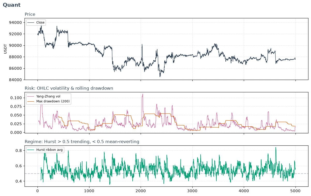
The professional-desk layer: volatility forecasting, risk sizing, regime detection, and factor construction. Where the retail indicators help you read a chart, these help you size a position, decide which strategy family fits the current regime, and build a cross-sectional book. Most are validated against real BTCUSDT market data rather than synthetic noise.
Volatility estimators
More accurate volatility than close-to-close, by using the whole OHLC bar. Each squeezes more information from the same data, trading off different assumptions:
historical_volatility— close-to-close baseline.parkinson_volatility— uses the high-low range; far more efficient, but assumes no drift or gaps.garman_klass_volatility— adds open/close to the range.rogers_satchell_volatility— unbiased under drift.yang_zhang_volatility— the desk favourite: handles both overnight gaps and drift. Reach for this when you have OHLC bars.ewma_volatility— RiskMetrics-style exponential weighting, so a vol spike shows immediately and fades smoothly instead of dropping off a cliffwindowbars later.
Risk-adjusted performance & tail risk
For position sizing — lean out as the tail fattens, not just as symmetric vol rises:
rolling_sharpe_ratio/rolling_sortino_ratio— return per unit of total / downside volatility.rolling_cvar— Conditional VaR / expected shortfall: the average of the worstαlosses. A coherent risk measure (unlike VaR), and the natural sizing denominator.cornish_fisher_var— VaR corrected for skew and fat tails, so it doesn't understate crash risk the way Gaussian VaR does.rolling_max_drawdown/calmar_ratio— worst peak-to-trough pain, and return earned per unit of it.
Distribution shape (regime fragility)
Higher moments turn before volatility does when a market becomes crash-prone:
rolling_skew/rolling_kurtosis— asymmetry and fat-tailedness.jarque_bera— one number summarising how non-Gaussian returns have been (rises when either tail asymmetry or fat tails appear).gain_to_pain— net move per unit of downside suffered; a robustness/smoothness screen.
Regime detection & signal conditioning
Decide which strategy family fits now, and make features usable:
hurst_ribbon— multi-scale Hurst exponent: trending (>0.5) vs. mean-reverting (<0.5) regime, at several horizons at once.regime_conditional_signal— a hard switch between two pre-built signals based on any regime score (e.g. trend-follow when Hurst says persistent, mean-revert otherwise).frac_diff— fractional differentiation (López de Prado): make a series stationary while keeping most of its memory — often the difference between a feature that predicts and a return series that doesn't.rolling_autocorr/rolling_ic— serial structure, and a feature's decaying predictive power (the IC is forward-looking — a monitoring diagnostic, never a live input).rolling_z_score/vol_adjusted_momentum/volatility_z_score/relative_volume— standardised / vol-scaled building blocks for gating and sizing.
Cross-sectional / factor plumbing
For a multi-asset book: compare symbols against each other, and against a
benchmark. Apply the cross-sectional ones with .over("timestamp") on a
long-format frame.
cross_sectional_zscore/cross_sectional_rank— rank symbols at each instant (the core of a factor strategy).momentum_12_1— the canonical Jegadeesh-Titman momentum factor (skip the last month to drop short-term reversal).rolling_beta_to/downside_beta— sensitivity to a benchmark, overall and in down markets (tail hedging).idiosyncratic_vol— the asset-specific risk a beta hedge leaves behind.amihud_illiquidity/micro_price_proxy— price impact per dollar traded, and a volume-tilted fair-price proxy.
rolling_sharpe_ratio(close: str, window: int = 63, risk_free_rate: float = 0.0) -> Expr
Annualized Rolling Sharpe Ratio (Assuming 252 trading days)
Source code in polars_ta/quant.py
117 118 119 120 121 122 123 124 125 126 127 128 129 130 | |
rolling_sortino_ratio(close: str, window: int = 63, risk_free_rate: float = 0.0) -> Expr
Annualized Rolling Sortino Ratio (Penalizes only downside volatility)
Source code in polars_ta/quant.py
133 134 135 136 137 138 139 140 141 142 143 144 145 146 147 | |
historical_volatility(close: str, window: int = 21) -> Expr
Annualized Historical Volatility (Close-to-Close)
Source code in polars_ta/quant.py
150 151 152 153 154 155 156 | |
ewma_volatility(close: str, window: int = 21, lambda_: float = 0.94) -> Expr
Annualized EWMA (RiskMetrics-style) volatility of log returns.
Unlike historical_volatility's flat rolling window, older squared
returns decay geometrically (weight lambda_ ** k), so a volatility
spike shows up immediately and fades out smoothly instead of dropping off
a cliff window bars later. lambda_=0.94 is the RiskMetrics daily
default; min_samples=window keeps the same warm-up convention as every
other volatility estimator here even though the EWM itself has infinite
memory.
Source code in polars_ta/quant.py
159 160 161 162 163 164 165 166 167 168 169 170 171 172 173 174 | |
parkinson_volatility(high: str, low: str, window: int = 20, trading_periods: int = 252) -> Expr
Parkinson (1980) high-low range volatility estimator, annualized.
Uses only the intraday high-low range, which makes it far more efficient than close-to-close historical volatility (it exploits the whole bar, not just the endpoints). It assumes no drift and no overnight jumps, so it complements Garman-Klass and Yang-Zhang rather than replacing them.
Source code in polars_ta/quant.py
177 178 179 180 181 182 183 184 185 186 187 188 189 190 191 192 193 194 195 | |
rogers_satchell_volatility(open_price: str, high: str, low: str, close: str, window: int = 20, trading_periods: int = 252) -> Expr
Rogers-Satchell (1991) volatility estimator, annualized.
Unlike Parkinson and Garman-Klass, this estimator is unbiased in the presence of a non-zero drift, using all four OHLC prices. It does not account for overnight gaps (that is what Yang-Zhang adds on top), so it is the natural mid-point of the OHLC-volatility family.
Source code in polars_ta/quant.py
198 199 200 201 202 203 204 205 206 207 208 209 210 211 212 213 214 215 216 217 218 219 220 221 222 223 224 225 | |
yang_zhang_volatility(open_price: str, high: str, low: str, close: str, window: int = 20, trading_periods: int = 252) -> Expr
Yang-Zhang (2000) volatility estimator, annualized.
Combines overnight (open-to-prev-close), open-to-close drift, and a Rogers-Satchell high/low term into a single minimum-variance estimator that (unlike close-to-close historical volatility or Garman-Klass) is unbiased in the presence of both overnight jumps and intraday drift. This is the volatility estimator of choice on professional vol desks when only OHLC bars (no tick data) are available.
Source code in polars_ta/quant.py
228 229 230 231 232 233 234 235 236 237 238 239 240 241 242 243 244 245 246 247 248 249 250 251 252 253 254 255 256 257 258 259 260 261 262 263 264 265 266 267 | |
hurst_ribbon(close: str, scales: tuple[int, ...] = (16, 32, 64)) -> dict[str, Expr]
Multi-scale Hurst ribbon: rescaled-range Hurst exponent computed at several window scales simultaneously, plus two derived regime features.
Returns a dict of expressions rather than a single one — pass its values
straight into with_columns(**hurst_ribbon("close").values()) or
unpack individual keys. Keys are h_{scale} for each scale, plus:
h_ribbon_avg: mean Hurst across scales — overall trending (>0.5) vs mean-reverting (<0.5) regime.h_ribbon_tilt: shortest-scale H minus longest-scale H — positive means short-term trend is stronger than long-term (breakout potential), negative means short-term is exhausting relative to the longer trend.
Unlike :func:hurst_exponent's full R/S analysis (accurate but
O(window) per row), this uses the cheap log(range/std)/log(window)
approximation, which is fast enough to run at several scales at once
and is the form used in production multi-scale regime detectors.
Source code in polars_ta/quant.py
270 271 272 273 274 275 276 277 278 279 280 281 282 283 284 285 286 287 288 289 290 291 292 293 294 295 296 297 298 299 300 301 302 303 304 305 306 307 | |
relative_volume(volume: str, window: int = 100) -> Expr
Relative volume (RVol): current volume vs its rolling mean.
Spikes in RVol often mark the start or end of a regime — a standard "is something happening right now" gate on execution/monitoring desks.
Source code in polars_ta/quant.py
310 311 312 313 314 315 316 317 | |
volatility_z_score(high: str, low: str, window: int = 100) -> Expr
Z-score of the rolling high-low range against its own recent history.
Flags volatility expansion/contraction relative to the recent norm, independent of the absolute price level — used to gate position sizing or strategy switching on a volatility-regime shift.
Source code in polars_ta/quant.py
320 321 322 323 324 325 326 327 328 329 330 331 332 333 334 | |
cross_sectional_zscore(value: str) -> Expr
Cross-sectional z-score of value at each timestamp.
Unlike every other indicator in this library, which computes a rolling
statistic through time for one symbol, this compares symbols against
each other at the same instant — the core building block of a
factor/ranking strategy. It is a per-symbol expression like any other,
but is only meaningful applied with .over(timestamp_column) on a
long-format multi-asset frame (columns: timestamp, symbol, value, ...),
grouping across symbols rather than across time:
df.with_columns(
    quant.cross_sectional_zscore("momentum").over("timestamp")
)
A cross-section with zero spread (all symbols tied) yields null rather than a divide-by-zero.
Source code in polars_ta/quant.py
337 338 339 340 341 342 343 344 345 346 347 348 349 350 351 352 353 354 355 356 357 358 359 | |
cross_sectional_rank(value: str, pct: bool = True) -> Expr
Cross-sectional rank of value at each timestamp, in [0, 1] by
default (pct=True) or as a dense integer rank (pct=False).
Same usage as :func:cross_sectional_zscore: apply with
.over(timestamp_column) on a long-format multi-asset frame to rank
symbols against each other at each instant, not through time.
Source code in polars_ta/quant.py
362 363 364 365 366 367 368 369 370 371 372 373 | |
amihud_illiquidity(close: str, volume: str, window: int = 21) -> Expr
Rolling Amihud Illiquidity (Price impact per dollar traded)
Source code in polars_ta/quant.py
376 377 378 379 380 381 382 383 384 385 386 387 388 389 390 | |
regime_conditional_signal(regime: str | Expr, threshold: float, signal_above: str | Expr, signal_below: str | Expr, above_or_equal: bool = True) -> Expr
Switch between two pre-computed signal expressions based on a
regime score, row by row: signal_above where regime >= threshold
(or > if above_or_equal=False), signal_below otherwise.
This is a hard switch, not a smooth blend — the output jumps discretely
at the threshold rather than fading between the two signals, which
keeps the composite as interpretable as its inputs (no intermediate
"40% trend-following" values to explain) at the cost of a
discontinuity exactly at the boundary. This is a compositional building
block, not a Hurst-specific helper: regime can be any expression —
quant.hurst_ribbon(...)["h_ribbon_avg"], an ADX reading, a Shannon
entropy score — and signal_above/signal_below can be any two
already-computed indicator expressions you want the regime to arbitrate
between (they are typically named differently, e.g. a fast EMA-cross
trend signal vs. a Bollinger %B mean-reversion signal — see the
"Regime-conditional trend/mean-reversion switch" how-to guide for a
complete example built on hurst_ribbon).
A null regime value produces a null output (arbitration is undefined
without a regime reading), rather than silently falling back to either
branch.
Source code in polars_ta/quant.py
393 394 395 396 397 398 399 400 401 402 403 404 405 406 407 408 409 410 411 412 413 414 415 416 417 418 419 420 421 422 423 424 425 426 427 428 429 430 431 432 433 434 | |
rolling_cvar(close: str | Expr, window: int = 100, alpha: float = 0.05) -> Expr
Rolling Conditional Value-at-Risk (Expected Shortfall) of simple returns.
CVaR at level alpha is the mean of the worst alpha fraction of
returns in the window — the expected loss given that the VaR threshold is
breached. Unlike VaR (a quantile), CVaR is a coherent risk measure
(sub-additive), which is why it is the tail metric of choice for position
sizing and the objective in Rockafellar-Uryasev portfolio optimization.
Reported as a positive loss magnitude (the sign is flipped), so larger
means more tail risk. A window with fewer than ceil(1/alpha) returns
can't resolve the alpha tail and reports null rather than a single-point
"expected shortfall".
Source code in polars_ta/quant.py
448 449 450 451 452 453 454 455 456 457 458 459 460 461 462 463 464 465 466 467 468 469 470 471 472 473 474 475 476 477 478 479 480 481 482 483 484 485 486 | |
cornish_fisher_var(close: str | Expr, window: int = 100, alpha: float = 0.05) -> Expr
Rolling Cornish-Fisher (modified) Value-at-Risk of simple returns.
Standard Gaussian VaR uses mu + z_alpha * sigma, which understates tail
risk for the negatively-skewed, fat-tailed return distributions typical of
risk assets. The Cornish-Fisher expansion corrects the Gaussian quantile
z for the sample skewness S and excess kurtosis K::
z_cf = z + (z^2-1)/6 * S + (z^3-3z)/24 * K - (2z^3-5z)/36 * S^2
and VaR = -(mu + z_cf * sigma), reported as a positive loss magnitude.
This is the RiskMetrics "modified VaR" and captures crash risk that
symmetric vol misses, without assuming a parametric fat-tailed family.
Source code in polars_ta/quant.py
489 490 491 492 493 494 495 496 497 498 499 500 501 502 503 504 505 506 507 508 509 510 511 512 513 514 515 516 517 518 519 520 521 522 523 524 525 | |
rolling_max_drawdown(close: str | Expr, window: int = 100) -> Expr
Rolling maximum drawdown over a trailing window of prices.
Drawdown at each bar is price / running_peak - 1; the maximum drawdown
over the window is the most negative such value, reported as a positive
fraction (e.g. 0.18 for an 18% peak-to-trough decline). Uses the
trailing rolling peak (rolling_max), so it is fully causal — no
look-ahead to a future high — and answers "how bad has the worst dip been
over the last window bars".
Source code in polars_ta/quant.py
528 529 530 531 532 533 534 535 536 537 538 539 540 541 542 | |
calmar_ratio(close: str | Expr, window: int = 252) -> Expr
Rolling Calmar ratio: annualized return divided by rolling max drawdown.
Calmar rewards return per unit of worst-case path pain rather than per
unit of volatility (Sharpe) — the metric managed-futures/CTA desks are
judged on, since it punishes a strategy that makes steady money then gives
it all back in one drawdown. Numerator is the annualized simple return over
the window ((P_t / P_{t-window})^{252/window} - 1); denominator is
:func:rolling_max_drawdown. A window with zero drawdown yields null (the
ratio is undefined, not infinite).
Source code in polars_ta/quant.py
545 546 547 548 549 550 551 552 553 554 555 556 557 558 559 560 561 562 563 564 | |
rolling_skew(close: str | Expr, window: int = 60) -> Expr
Rolling skewness of simple returns over window bars.
Persistent negative skew ("picks up pennies in front of a steamroller") is the classic signature of a strategy or regime carrying hidden crash risk; rising positive skew often accompanies momentum/blow-off phases. A zero-dispersion window (constant returns) has undefined skew and yields null rather than leaking NaN.
Source code in polars_ta/quant.py
578 579 580 581 582 583 584 585 586 587 588 | |
rolling_kurtosis(close: str | Expr, window: int = 60) -> Expr
Rolling excess kurtosis of simple returns over window bars.
Excess kurtosis (normal distribution -> 0) rising well above 0 flags
fat tails / clustered extreme moves — a warning that Gaussian VaR and any
downstream mean-variance sizing are understating tail risk. Pairs naturally
with :func:cornish_fisher_var, which uses exactly this moment. A
zero-dispersion window (constant returns) has undefined kurtosis and yields
null rather than leaking NaN.
Source code in polars_ta/quant.py
591 592 593 594 595 596 597 598 599 600 601 602 603 604 605 606 | |
gain_to_pain(close: str | Expr, window: int = 60) -> Expr
Rolling gain-to-pain ratio: sum of returns divided by sum of losses.
Defined (Schwager) as sum(returns) / sum(|negative returns|) over the
window — total net move per unit of downside suffered. It is more robust
than Sharpe to a handful of outlier winners (it doesn't reward upside
volatility at all) and is a standard discretionary-desk screen for
"smoothness" of a return stream. A window with no losing bars yields null
(infinite gain-to-pain is not a meaningful finite feature).
Source code in polars_ta/quant.py
609 610 611 612 613 614 615 616 617 618 619 620 621 622 623 | |
jarque_bera(close: str | Expr, window: int = 60) -> Expr
Rolling Jarque-Bera normality test statistic of simple returns.
JB = (n / 6) * (S**2 + K**2 / 4) where S is the skewness and K
the excess kurtosis of the returns in the window. Under the null of
normally distributed returns JB is asymptotically chi-squared with 2
degrees of freedom, so a value above ~6 rejects normality at the 5% level
(~9.2 at 1%). It is a single scalar that rises when either tail asymmetry
or fat-tailedness appears — a compact "how non-Gaussian has this regime
been" gate that subsumes :func:rolling_skew and :func:rolling_kurtosis
into one number, which matters because any downstream Gaussian VaR /
mean-variance sizing is only valid while JB stays small.
Reuses the same biased (population) moments Polars' rolling_skew /
rolling_kurtosis report, so it is consistent with those two features
rather than a separately-normalized estimate.
Source code in polars_ta/quant.py
626 627 628 629 630 631 632 633 634 635 636 637 638 639 640 641 642 643 644 645 646 647 648 | |
frac_diff(close: str | Expr, d: float = 0.4, window: int = 100) -> Expr
Fixed-width-window fractional differentiation of the log price.
Applies the binomial fractional-difference operator (1-L)^d truncated
to a fixed window (Lopez de Prado, Advances in Financial ML, ch. 5).
For d in (0, 1) the output is (approximately) stationary while
retaining far more of the original series' long memory than a full first
difference (d = 1, ordinary log returns) would — often the difference
between a feature that passes an ADF stationarity test and still predicts,
versus a return series that is stationary but has thrown its memory away.
Weights w_k = -w_{k-1} (d-k+1)/k are applied to the trailing window
log-prices. Larger d -> more differencing / less memory; d near 0
keeps almost all memory but may not fully stationarize.
Source code in polars_ta/quant.py
670 671 672 673 674 675 676 677 678 679 680 681 682 683 684 685 686 687 688 689 690 691 692 | |
rolling_autocorr(close: str | Expr, lag: int = 1, window: int = 60) -> Expr
Rolling lag-lag autocorrelation of simple returns.
corr(r_t, r_{t-lag}) over a trailing window. Positive lag-1
autocorrelation is momentum/trending structure; negative is mean reversion
(bid-ask bounce at short horizons, or genuine reversal at longer ones). A
direct, sign-explicit complement to the variance ratio and Hurst tools. A
flat window (zero variance) yields null.
Source code in polars_ta/quant.py
695 696 697 698 699 700 701 702 703 704 705 706 707 708 709 710 711 712 | |
rolling_ic(signal: str | Expr, forward_return: str | Expr, window: int = 60) -> Expr
Rolling information coefficient: correlation between a signal and the realized forward return.
The IC is the single most important diagnostic for a predictive feature:
the rolling Pearson correlation between signal_t and the
contemporaneous forward_return_t column (which you construct as a
forward return, e.g. close.pct_change().shift(-h), so that at
evaluation time the pair (signal_t, fwd_ret_t) is aligned). A decaying
rolling IC is the earliest sign of alpha decay — the feature has stopped
working — long before the equity curve rolls over.
Look-ahead warning: forward_return is forward-looking by
construction; that is correct for measuring predictive power but means the
IC series itself must never be used as a live trading input — it is a
research/monitoring diagnostic. A flat window yields null.
Source code in polars_ta/quant.py
715 716 717 718 719 720 721 722 723 724 725 726 727 728 729 730 731 732 733 734 735 736 737 738 739 740 | |
rolling_beta_to(close: str | Expr, benchmark: str | Expr, window: int = 60) -> Expr
Rolling market beta of an asset's returns against a benchmark's returns.
OLS slope of the asset's simple returns on the benchmark's simple returns
over a trailing window — the sensitivity a factor-neutral book needs to
hedge out. benchmark is a returns-bearing price column (e.g. BTC or an
index level) carried alongside the asset on the same frame. A flat
benchmark window yields null.
Source code in polars_ta/quant.py
754 755 756 757 758 759 760 761 762 763 764 765 766 767 | |
idiosyncratic_vol(close: str | Expr, benchmark: str | Expr, window: int = 60) -> Expr
Rolling idiosyncratic (residual) volatility relative to a benchmark.
The part of an asset's return variance the benchmark does not explain:
sqrt(var(r_asset) * (1 - rho^2)) over the window, where rho is the
rolling correlation to the benchmark. This is the risk that survives a
beta hedge — the tradeable, asset-specific component a stat-arb/relative-
value book actually harvests, and a cleaner "specialness" measure than raw
volatility. Annualized by sqrt(252).
Source code in polars_ta/quant.py
770 771 772 773 774 775 776 777 778 779 780 781 782 783 784 785 786 787 788 789 790 791 792 793 | |
downside_beta(close: str | Expr, benchmark: str | Expr, window: int = 60) -> Expr
Rolling downside beta: beta estimated only on bars where the benchmark fell.
Bawa-Lindenberg / Ang-Chen downside beta captures how an asset behaves when the market is down — the regime that actually matters for tail hedging and that symmetric beta averages away. Computed as the OLS slope of asset returns on benchmark returns restricted to benchmark-negative bars within each trailing window. A window with fewer than two down-benchmark bars (or a flat down-benchmark subset) yields null.
Unlike the symmetric :func:rolling_beta_to, the down-bar subset can't use
the shared rolling-covariance primitive (its windows would be riddled with
the masked-out up-bars, and Polars' default rolling requires a full window
of non-nulls), so the per-window OLS on the down subset runs in a single
map_batches pass over a stacked [asset, bench] struct.
Source code in polars_ta/quant.py
796 797 798 799 800 801 802 803 804 805 806 807 808 809 810 811 812 813 814 815 816 817 818 819 820 821 822 823 824 825 826 827 828 829 830 831 832 833 834 835 836 837 838 839 840 841 842 843 844 845 846 | |
momentum_12_1(close: str | Expr, lookback: int = 252, skip: int = 21) -> Expr
Cross-sectional price momentum, skipping the most recent skip bars.
The canonical Jegadeesh-Titman / Fama-French "momentum 12-1" factor: the
return from lookback bars ago up to skip bars ago
(P_{t-skip} / P_{t-lookback} - 1), deliberately excluding the most
recent month. The skip removes the well-documented short-term reversal
(bid-ask bounce and 1-month mean reversion) that otherwise contaminates the
momentum signal. Feed the result through :func:cross_sectional_rank or
:func:cross_sectional_zscore .over(timestamp) to build the ranked
factor.
Source code in polars_ta/quant.py
849 850 851 852 853 854 855 856 857 858 859 860 861 862 863 864 | |