Skip to content

Microstructure

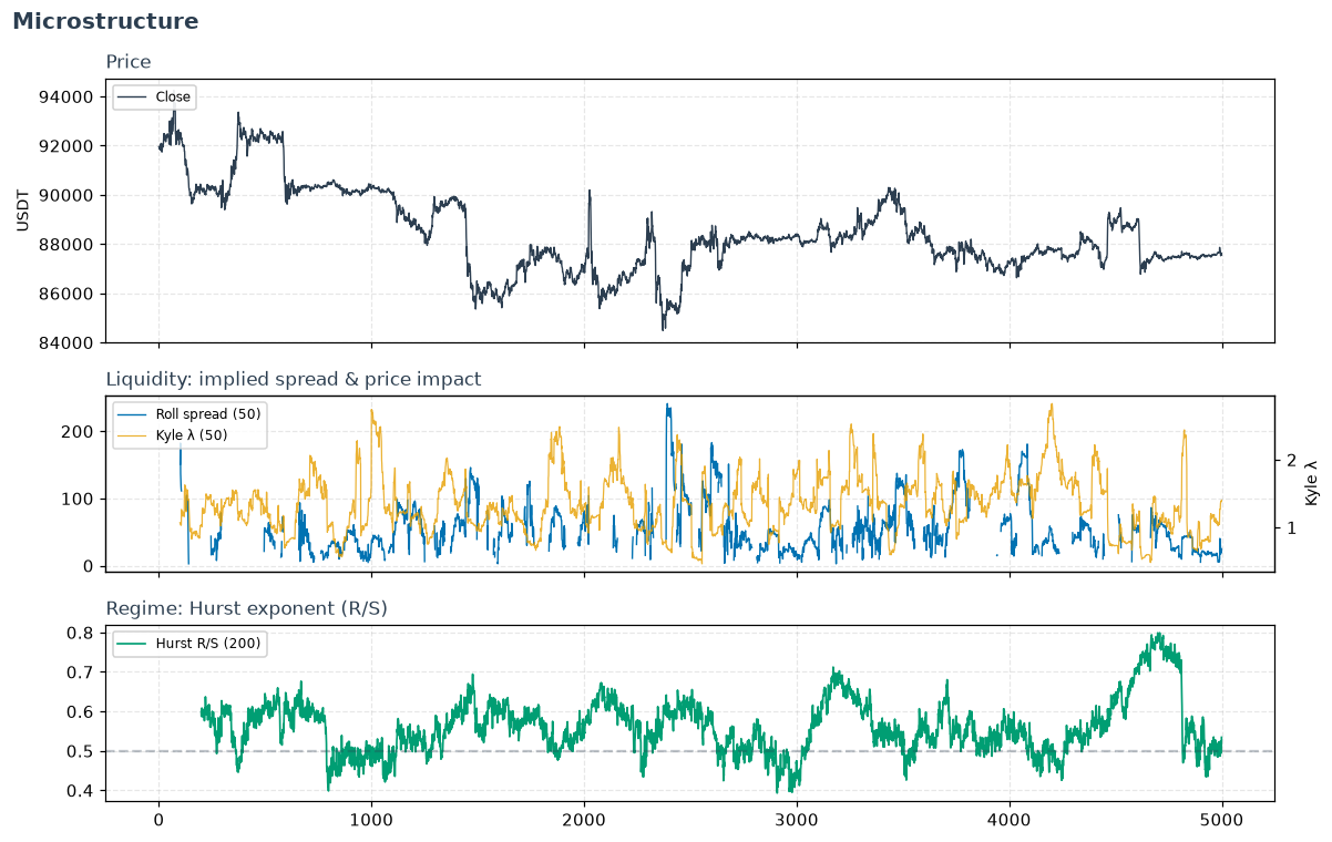
Price, Roll spread with Kyle's lambda, and the Hurst R/S regime line on BTCUSDT 5m

How the market is trading underneath the price — liquidity, the cost of crossing the spread, whether order flow looks informed, and how fast a series reverts. These are standard on institutional desks and largely absent from retail TA libraries, because they need bar-level volume classification, autocovariance of returns, or scaling-law fits rather than a simple rolling window. All are validated against real BTCUSDT data.

Spread & transaction cost (from prices alone)

Recover the effective bid-ask spread without quote data:

  • roll_spread — Roll (1984), from the negative autocovariance that bid-ask bounce induces in price changes.
  • corwin_schultz_spread — the modern high-low estimator; more robust on OHLC bars than Roll.
  • effective_spread — distance of the trade price from the mid.

Price impact & liquidity

How much price moves per unit of order flow — thinner market, steeper impact:

  • kyle_lambda — Kyle (1985): the workhorse linear price-impact measure for sizing orders against liquidity.
  • hasbrouck_lambda — impact in log-price / √dollar-volume space, matching the empirical square-root impact law.

Order-flow toxicity & trade direction

  • vpin — Volume-Synchronised Probability of Informed Trading: order-flow imbalance in volume time, the canonical flow-toxicity warning (it spiked ahead of the 2010 Flash Crash).
  • lee_ready_trade_sign — classifies each trade as buy- or sell-initiated (the input to signed-flow measures).

Regime & mean-reversion diagnostics

Decide whether to run momentum or mean-reversion, and how fast reversion is:

  • hurst_exponent — full R/S Hurst: persistent (>0.5) vs. mean-reverting (<0.5). (For a fast multi-scale version, see quant.hurst_ribbon.)
  • half_life — how many bars a mean-reverting series takes to close half the gap to its mean (from an OU fit). The "how fast does it revert?" number for stat-arb.
  • variance_ratio — Lo-MacKinlay test: is this a random walk (=1), trending (>1), or mean-reverting (<1)?
  • shannon_entropy / approximate_entropy — distributional complexity and pattern predictability; complementary to Hurst (they don't care about direction, only structure).

These describe conditions, not signals

Microstructure tools are for classifying the environment — is it liquid, is flow toxic, is it trending or reverting — and gating strategy choice, rather than firing buy/sell signals directly.


polars_ta.microstructure

Market microstructure and order-flow features used on professional/quant desks.

These are largely absent from retail TA libraries (they need bar-level volume classification, autocovariance of returns, or scaling-law fits rather than a simple rolling window), but are standard tools for liquidity analysis, informed-trading detection, and regime classification on institutional desks.

roll_spread

roll_spread(close: str | Expr, window: int = 20) -> Expr

Roll (1984) implied bid-ask spread from serial covariance of price changes.

Estimates the effective spread purely from trade prices, using the fact that bid-ask bounce induces negative first-order autocovariance in price changes: spread = 2 * sqrt(-cov(delta_p_t, delta_p_t-1)) when that covariance is negative (as microstructure theory predicts); the window is reported as null when the covariance is non-negative, since the model's premise doesn't hold there.

Source code in polars_ta/microstructure.py
 89
 90
 91
 92
 93
 94
 95
 96
 97
 98
 99
100
101
102
103
104
105
def roll_spread(close: str | pl.Expr, window: int = 20) -> pl.Expr:
    """Roll (1984) implied bid-ask spread from serial covariance of price changes.

    Estimates the effective spread purely from trade prices, using the fact
    that bid-ask bounce induces negative first-order autocovariance in price
    changes: spread = 2 * sqrt(-cov(delta_p_t, delta_p_t-1)) when that
    covariance is negative (as microstructure theory predicts); the window
    is reported as null when the covariance is non-negative, since the
    model's premise doesn't hold there.
    """
    close = as_expr(close)
    delta_p = close.diff(1)

    cov = rolling_cov(delta_p, delta_p.shift(1), window)

    spread = pl.when(cov < 0).then(2.0 * (-cov).sqrt()).otherwise(None)
    return spread.alias(f"roll_spread_{window}")

kyle_lambda

kyle_lambda(close: str | Expr, volume: str | Expr, window: int = 20) -> Expr

Kyle's (1985) lambda: price impact per unit of signed order flow.

Regresses price changes on signed volume (sign of the price change used as a trade-direction proxy, i.e. a tick rule) within a rolling window. A steeper slope means the market absorbs less volume per unit of price move — thinner, less liquid conditions. This is the workhorse price-impact measure for execution/market-making desks sizing orders against liquidity.

Source code in polars_ta/microstructure.py
108
109
110
111
112
113
114
115
116
117
118
119
120
121
122
123
124
125
126
def kyle_lambda(
    close: str | pl.Expr, volume: str | pl.Expr, window: int = 20
) -> pl.Expr:
    """Kyle's (1985) lambda: price impact per unit of signed order flow.

    Regresses price changes on signed volume (sign of the price change used
    as a trade-direction proxy, i.e. a tick rule) within a rolling window.
    A steeper slope means the market absorbs less volume per unit of price
    move — thinner, less liquid conditions. This is the workhorse price-impact
    measure for execution/market-making desks sizing orders against liquidity.
    """
    close = as_expr(close)
    volume = as_expr(volume)

    delta_p = close.diff(1)
    signed_volume = volume * delta_p.sign()

    # Slope of price change on signed volume: cov(sv, dp) / var(sv).
    return rolling_beta(delta_p, signed_volume, window).alias(f"kyle_lambda_{window}")

hasbrouck_lambda

hasbrouck_lambda(close: str | Expr, volume: str | Expr, window: int = 20) -> Expr

Hasbrouck's (1991) lambda: price impact regressed in log-price / sqrt(dollar-volume) space rather than Kyle's raw price/volume space.

Using sqrt(signed dollar volume) makes the impact measure robust to the typical square-root law of market impact, which is closer to what execution desks actually observe versus Kyle's linear assumption.

Source code in polars_ta/microstructure.py
129
130
131
132
133
134
135
136
137
138
139
140
141
142
143
144
145
146
147
148
149
def hasbrouck_lambda(
    close: str | pl.Expr, volume: str | pl.Expr, window: int = 20
) -> pl.Expr:
    """Hasbrouck's (1991) lambda: price impact regressed in log-price /
    sqrt(dollar-volume) space rather than Kyle's raw price/volume space.

    Using sqrt(signed dollar volume) makes the impact measure robust to the
    typical square-root law of market impact, which is closer to what
    execution desks actually observe versus Kyle's linear assumption.
    """
    close = as_expr(close)
    volume = as_expr(volume)

    log_ret = log_return(close)
    dollar_volume = close * volume
    signed_sqrt_dv = dollar_volume.sqrt() * log_ret.sign()

    # Slope of log return on signed sqrt dollar volume.
    return rolling_beta(log_ret, signed_sqrt_dv, window).alias(
        f"hasbrouck_lambda_{window}"
    )

effective_spread

effective_spread(close: str | Expr, mid_price: str | Expr | None = None) -> Expr

Effective spread proxy: 2 * |close - mid|, in the same units as price.

When no explicit mid-price/quote data is available (the common case for bar data), the previous close is used as a proxy for the prevailing mid, which is the standard fallback in the academic microstructure literature when only trade prices are observable.

Source code in polars_ta/microstructure.py
152
153
154
155
156
157
158
159
160
161
162
163
164
165
166
167
def effective_spread(
    close: str | pl.Expr, mid_price: str | pl.Expr | None = None
) -> pl.Expr:
    """Effective spread proxy: 2 * |close - mid|, in the same units as price.

    When no explicit mid-price/quote data is available (the common case for
    bar data), the previous close is used as a proxy for the prevailing mid,
    which is the standard fallback in the academic microstructure literature
    when only trade prices are observable.
    """
    close = as_expr(close)
    if mid_price is None:
        mid = close.shift(1)
    else:
        mid = as_expr(mid_price)
    return (2.0 * (close - mid).abs()).alias("effective_spread")

lee_ready_trade_sign

lee_ready_trade_sign(close: str | Expr, mid_price: str | Expr | None = None) -> Expr

Lee-Ready trade-side classification: +1 buy-initiated, -1 sell-initiated, 0 unclassifiable, per bar/trade.

The full Lee & Ready (1991) algorithm classifies by the quote test (trade price vs. the prevailing bid-ask midpoint) first, falling back to the tick test (trade price vs. the previous trade price) only when the trade is exactly at the midpoint. Bar data has no quotes, so when mid_price isn't supplied the quote test is skipped entirely (comparing close against its own previous value as "mid" would make the quote test degenerate into the tick test) and classification falls straight to the tick test — the standard reduction used when only trade prices are observable. A genuine tie (flat price) is unclassifiable (0), never guessed.

Source code in polars_ta/microstructure.py
170
171
172
173
174
175
176
177
178
179
180
181
182
183
184
185
186
187
188
189
190
191
192
193
194
195
196
197
198
199
200
201
202
def lee_ready_trade_sign(
    close: str | pl.Expr, mid_price: str | pl.Expr | None = None
) -> pl.Expr:
    """Lee-Ready trade-side classification: +1 buy-initiated, -1
    sell-initiated, 0 unclassifiable, per bar/trade.

    The full Lee & Ready (1991) algorithm classifies by the quote test
    (trade price vs. the prevailing bid-ask midpoint) first, falling back to
    the tick test (trade price vs. the previous trade price) only when the
    trade is exactly at the midpoint. Bar data has no quotes, so when
    `mid_price` isn't supplied the quote test is skipped entirely (comparing
    close against its own previous value as "mid" would make the quote test
    degenerate into the tick test) and classification falls straight to the
    tick test — the standard reduction used when only trade prices are
    observable. A genuine tie (flat price) is unclassifiable (`0`), never
    guessed.
    """
    close = as_expr(close)
    prev_close = close.shift(1)
    tick_sign = (
        pl.when(close > prev_close)
        .then(1)
        .when(close < prev_close)
        .then(-1)
        .otherwise(None)
    )

    if mid_price is None:
        return tick_sign.fill_null(0).alias("trade_sign")

    mid = as_expr(mid_price)
    quote_sign = pl.when(close > mid).then(1).when(close < mid).then(-1).otherwise(None)
    return quote_sign.fill_null(tick_sign).fill_null(0).alias("trade_sign")

vpin

vpin(close: str | Expr, volume: str | Expr, bucket_size: int, window: int = 50) -> Expr

Volume-Synchronized Probability of Informed Trading (Easley, Lopez de Prado & O'Hara, 2012).

Bars are aggregated into equal-sized volume buckets (not time bars), each bucket's volume is split into buy/sell using bulk volume classification (a z-scored price-change CDF, standard for bar data without tick-level trade direction), and VPIN is the rolling mean of |buy - sell| / total volume across the last window buckets. High VPIN signals order-flow imbalance consistent with informed trading — the canonical warning signal ahead of liquidity-driven crashes (e.g. the 2010 Flash Crash), used on institutional desks for flow-toxicity monitoring rather than directional signal generation.

Parameters:

Name Type Description Default
bucket_size int

total volume per synchronized bucket (must match the typical scale of volume for the instrument).

required
window int

number of trailing buckets averaged into the VPIN estimate.

50
Source code in polars_ta/microstructure.py
205
206
207
208
209
210
211
212
213
214
215
216
217
218
219
220
221
222
223
224
225
226
227
228
229
230
231
232
233
234
235
236
237
238
239
240
241
242
243
244
245
246
247
248
249
250
251
252
253
254
255
256
257
258
259
260
261
262
263
264
265
266
267
268
269
270
271
272
273
274
275
276
277
278
279
280
281
282
283
284
285
286
287
288
def vpin(
    close: str | pl.Expr,
    volume: str | pl.Expr,
    bucket_size: int,
    window: int = 50,
) -> pl.Expr:
    """Volume-Synchronized Probability of Informed Trading (Easley, Lopez de
    Prado & O'Hara, 2012).

    Bars are aggregated into equal-sized *volume buckets* (not time bars),
    each bucket's volume is split into buy/sell using bulk volume
    classification (a z-scored price-change CDF, standard for bar data
    without tick-level trade direction), and VPIN is the rolling mean of
    |buy - sell| / total volume across the last `window` buckets. High VPIN
    signals order-flow imbalance consistent with informed trading — the
    canonical warning signal ahead of liquidity-driven crashes (e.g. the
    2010 Flash Crash), used on institutional desks for flow-toxicity
    monitoring rather than directional signal generation.

    Args:
        bucket_size: total volume per synchronized bucket (must match the
            typical scale of `volume` for the instrument).
        window: number of trailing buckets averaged into the VPIN estimate.
    """
    close = as_expr(close)
    volume = as_expr(volume)

    def _calc_vpin(struct_s: pl.Series) -> pl.Series:
        df = struct_s.struct.unnest()
        price = df["close"].to_numpy()
        vol = df["volume"].to_numpy()
        n = len(price)

        ret = np.diff(price, prepend=price[0])
        std = np.nanstd(ret) if np.nanstd(ret) > 0 else 1.0
        z = ret / std
        # Standard normal CDF via erf (bulk volume classification, Easley et al.)
        buy_frac = 0.5 * (1.0 + np.vectorize(math.erf)(z / math.sqrt(2.0)))

        # The volume-bucketing accumulator is the one genuinely sequential
        # step; hand it to the (optionally Numba-compiled) kernel. Everything
        # around it — classification above, rolling mean below — is vectorized.
        buy_arr, sell_arr, bucket_idx = _vpin_bucketing(
            np.ascontiguousarray(vol, dtype=np.float64),
            np.ascontiguousarray(buy_frac, dtype=np.float64),
            float(bucket_size),
        )

        if len(buy_arr) == 0:
            return pl.Series([None] * n, dtype=pl.Float64)

        imbalance = np.abs(buy_arr - sell_arr)
        total = buy_arr + sell_arr
        safe_total = np.where(total == 0, np.nan, total)
        oi = imbalance / safe_total

        # Trailing rolling mean over the last `window` buckets, ignoring
        # zero-total buckets (NaN in `oi`) — vectorized via a sliding-window
        # view instead of a per-bucket Python loop. The first window-1 buckets
        # stay NaN (not enough history yet).
        vpin_buckets = np.full(len(oi), np.nan)
        if len(oi) >= window:
            windows = np.lib.stride_tricks.sliding_window_view(oi, window)
            with np.errstate(invalid="ignore"):
                means = np.where(
                    np.isnan(windows).all(axis=1),
                    np.nan,
                    np.nanmean(windows, axis=1),
                )
            vpin_buckets[window - 1 :] = means

        # Broadcast each bucket's VPIN back onto its member bars via fancy
        # indexing. Bars in the trailing, not-yet-filled bucket carry
        # bucket_idx == -1 and stay null (how every indicator signals "not
        # enough data yet").
        out = np.full(n, np.nan)
        valid = (bucket_idx >= 0) & (bucket_idx < len(vpin_buckets))
        out[valid] = vpin_buckets[bucket_idx[valid]]
        return pl.Series(out, dtype=pl.Float64).fill_nan(None)

    expr = pl.struct([close.alias("close"), volume.alias("volume")]).map_batches(
        _calc_vpin, returns_scalar=False
    )
    return expr.alias(f"vpin_{bucket_size}_{window}")

hurst_exponent

hurst_exponent(close: str | Expr, window: int = 100) -> Expr

Rolling Hurst exponent via rescaled-range (R/S) analysis.

H < 0.5 indicates a mean-reverting regime, H = 0.5 a random walk, and H > 0.5 a trending/persistent regime. Quant desks use this to switch strategy family (momentum vs mean-reversion) rather than as a trade signal by itself.

Implemented with a single map_batches pass and a sliding-window view (no per-row Python rolling_map): each window's R/S regression is computed over NumPy-reshaped chunks, so cost is dominated by vectorized array ops rather than an O(window) Python loop per row.

Source code in polars_ta/microstructure.py
330
331
332
333
334
335
336
337
338
339
340
341
342
343
344
345
346
347
348
349
350
351
352
353
354
355
356
357
358
359
360
def hurst_exponent(close: str | pl.Expr, window: int = 100) -> pl.Expr:
    """Rolling Hurst exponent via rescaled-range (R/S) analysis.

    H < 0.5 indicates a mean-reverting regime, H = 0.5 a random walk, and
    H > 0.5 a trending/persistent regime. Quant desks use this to switch
    strategy family (momentum vs mean-reversion) rather than as a trade
    signal by itself.

    Implemented with a single ``map_batches`` pass and a sliding-window view
    (no per-row Python ``rolling_map``): each window's R/S regression is
    computed over NumPy-reshaped chunks, so cost is dominated by vectorized
    array ops rather than an O(window) Python loop per row.
    """
    close = as_expr(close)
    log_ret = log_return(close)

    def _rolling_hurst(s: pl.Series) -> pl.Series:
        x = s.to_numpy()
        n = len(x)
        out = np.full(n, np.nan)
        if n < window:
            return pl.Series(out, dtype=pl.Float64).fill_nan(None)
        # Sliding windows as a zero-copy view; evaluate R/S per window.
        views = np.lib.stride_tricks.sliding_window_view(x, window)
        for i in range(views.shape[0]):
            out[window - 1 + i] = _hurst_from_window(views[i])
        return pl.Series(out, dtype=pl.Float64).fill_nan(None)

    return log_ret.map_batches(_rolling_hurst, returns_scalar=False).alias(
        f"hurst_{window}"
    )

variance_ratio

variance_ratio(close: str | Expr, window: int = 20, lag: int = 2) -> Expr

Lo-MacKinlay (1988) variance ratio test statistic, rolled over window.

VR(lag) = Var(lag-period return) / (lag * Var(1-period return)). Under the random-walk null hypothesis VR = 1; VR > 1 indicates positive serial correlation (trending), VR < 1 indicates mean reversion. Used by quant desks to test whether a random-walk assumption (and therefore standard options-pricing / risk models built on it) actually holds for an instrument over a given regime.

Source code in polars_ta/microstructure.py
363
364
365
366
367
368
369
370
371
372
373
374
375
376
377
378
379
380
381
382
def variance_ratio(close: str | pl.Expr, window: int = 20, lag: int = 2) -> pl.Expr:
    """Lo-MacKinlay (1988) variance ratio test statistic, rolled over `window`.

    VR(lag) = Var(lag-period return) / (lag * Var(1-period return)). Under
    the random-walk null hypothesis VR = 1; VR > 1 indicates positive serial
    correlation (trending), VR < 1 indicates mean reversion. Used by quant
    desks to test whether a random-walk assumption (and therefore standard
    options-pricing / risk models built on it) actually holds for an
    instrument over a given regime.
    """
    close = as_expr(close)
    ret_1 = log_return(close, periods=1)
    ret_lag = log_return(close, periods=lag)

    var_1 = ret_1.rolling_var(window_size=window)
    var_lag = ret_lag.rolling_var(window_size=window)

    safe_var_1 = pl.when(var_1 == 0).then(None).otherwise(var_1)
    vr = var_lag / (lag * safe_var_1)
    return vr.alias(f"variance_ratio_{lag}_{window}")

corwin_schultz_spread

corwin_schultz_spread(high: str | Expr, low: str | Expr, window: int = 20) -> Expr

Corwin-Schultz (2012) high-low bid-ask spread estimator.

Recovers the effective spread from two consecutive daily high-low ranges only (no volume, no quotes). The insight is that the high-low range reflects both the true variance (which scales with the time interval) and the spread (which does not), so combining a single-bar range with a two-bar range separates the two. This is the modern successor to Roll's estimator and is far more robust on OHLC bar data; negative per-bar estimates (which the model treats as zero spread) are floored at zero and the result is averaged over window bars.

Source code in polars_ta/microstructure.py
385
386
387
388
389
390
391
392
393
394
395
396
397
398
399
400
401
402
403
404
405
406
407
408
409
410
411
412
413
414
415
416
417
418
def corwin_schultz_spread(
    high: str | pl.Expr, low: str | pl.Expr, window: int = 20
) -> pl.Expr:
    """Corwin-Schultz (2012) high-low bid-ask spread estimator.

    Recovers the effective spread from two consecutive daily high-low ranges
    only (no volume, no quotes). The insight is that the high-low range
    reflects both the true variance (which scales with the time interval) and
    the spread (which does not), so combining a single-bar range with a
    two-bar range separates the two. This is the modern successor to Roll's
    estimator and is far more robust on OHLC bar data; negative per-bar
    estimates (which the model treats as zero spread) are floored at zero and
    the result is averaged over ``window`` bars.
    """
    high = as_expr(high)
    low = as_expr(low)

    # beta: sum of two consecutive single-bar squared log high/low ranges.
    hl = (high / low).log().pow(2)
    beta = hl + hl.shift(1)

    # gamma: squared log range over the two-bar high and two-bar low.
    high2 = pl.max_horizontal(high, high.shift(1))
    low2 = pl.min_horizontal(low, low.shift(1))
    gamma = (high2 / low2).log().pow(2)

    denom = 3.0 - 2.0 * math.sqrt(2.0)
    alpha = (beta.sqrt() * (math.sqrt(2.0) - 1.0) / denom) - (gamma / denom).sqrt()

    # Spread as a fraction of price; negative alpha -> zero spread.
    ea = alpha.exp()
    spread = 2.0 * (ea - 1.0) / (1.0 + ea)
    spread = pl.when(spread < 0).then(0.0).otherwise(spread)
    return spread.rolling_mean(window_size=window).alias(f"corwin_schultz_{window}")

half_life

half_life(close: str | Expr, window: int = 60) -> Expr

Half-life of mean reversion from a rolling Ornstein-Uhlenbeck fit.

Regresses the change in price on the lagged price level within each window (an AR(1) / discretized OU fit): dP_t = a + b * P_{t-1}. When b < 0 the series is mean-reverting and the half-life — the expected number of bars to close half the gap to the mean — is -ln(2) / ln(1+b). Non-mean-reverting windows (b >= 0) are reported as null. This is the workhorse "how fast does it revert" number on stat-arb desks, pairing naturally with :func:variance_ratio and :func:hurst_exponent.

Source code in polars_ta/microstructure.py
421
422
423
424
425
426
427
428
429
430
431
432
433
434
435
436
437
438
439
440
441
def half_life(close: str | pl.Expr, window: int = 60) -> pl.Expr:
    """Half-life of mean reversion from a rolling Ornstein-Uhlenbeck fit.

    Regresses the change in price on the lagged price level within each
    window (an AR(1) / discretized OU fit): ``dP_t = a + b * P_{t-1}``. When
    ``b < 0`` the series is mean-reverting and the half-life — the expected
    number of bars to close half the gap to the mean — is ``-ln(2) / ln(1+b)``.
    Non-mean-reverting windows (``b >= 0``) are reported as null. This is the
    workhorse "how fast does it revert" number on stat-arb desks, pairing
    naturally with :func:`variance_ratio` and :func:`hurst_exponent`.
    """
    close = as_expr(close)
    y = close.diff(1)  # dP_t
    x = close.shift(1)  # P_{t-1}

    # AR(1) slope b in dP_t = a + b * P_{t-1}.
    b = rolling_beta(y, x, window)
    # Only mean-reverting fits (b in (-1, 0)) yield a finite positive half-life.
    valid = (b < 0) & (b > -1)
    hl = pl.when(valid).then(-math.log(2) / (1.0 + b).log()).otherwise(None)
    return hl.alias(f"half_life_{window}")

shannon_entropy

shannon_entropy(close: str | Expr, window: int = 50, n_bins: int = 10) -> Expr

Rolling Shannon entropy (normalized to [0, 1]) of the binned distribution of log returns within each window.

A value near 1 means returns within the window are spread roughly uniformly across bins — high "surprise"/complexity, consistent with a noisy or regime-shifting market. A value near 0 means returns cluster into a few bins — low complexity, consistent with a persistent trend or a tightly range-bound market. Unlike the Hurst exponent (which measures directional persistence), entropy measures distributional concentration and doesn't care about sign or serial correlation, so the two are complementary regime signals rather than redundant ones.

A window with fewer non-null returns than n_bins can't populate every bin meaningfully and reports null rather than a misleadingly low entropy.

Source code in polars_ta/microstructure.py
458
459
460
461
462
463
464
465
466
467
468
469
470
471
472
473
474
475
476
477
478
479
480
481
482
483
484
485
486
487
488
489
490
491
492
def shannon_entropy(
    close: str | pl.Expr, window: int = 50, n_bins: int = 10
) -> pl.Expr:
    """Rolling Shannon entropy (normalized to [0, 1]) of the binned
    distribution of log returns within each window.

    A value near 1 means returns within the window are spread roughly
    uniformly across bins — high "surprise"/complexity, consistent with a
    noisy or regime-shifting market. A value near 0 means returns cluster
    into a few bins — low complexity, consistent with a persistent trend or
    a tightly range-bound market. Unlike the Hurst exponent (which measures
    *directional persistence*), entropy measures *distributional
    concentration* and doesn't care about sign or serial correlation, so the
    two are complementary regime signals rather than redundant ones.

    A window with fewer non-null returns than `n_bins` can't populate every
    bin meaningfully and reports null rather than a misleadingly low entropy.
    """
    close = as_expr(close)
    log_ret = log_return(close)

    def _rolling_entropy(s: pl.Series) -> pl.Series:
        x = s.to_numpy()
        n = len(x)
        out = np.full(n, np.nan)
        if n < window:
            return pl.Series(out, dtype=pl.Float64).fill_nan(None)
        views = np.lib.stride_tricks.sliding_window_view(x, window)
        for i in range(views.shape[0]):
            out[window - 1 + i] = _shannon_entropy_from_window(views[i], n_bins)
        return pl.Series(out, dtype=pl.Float64).fill_nan(None)

    return log_ret.map_batches(_rolling_entropy, returns_scalar=False).alias(
        f"shannon_entropy_{window}"
    )

approximate_entropy

approximate_entropy(close: str | Expr, window: int = 30, m: int = 2, r_frac: float = 0.2) -> Expr

Rolling approximate entropy (ApEn) of log returns within each window.

Measures how predictable consecutive m-length patterns are: low ApEn means the series repeats similar short patterns (more regular/ predictable), high ApEn means patterns rarely recur (more random). r (the similarity tolerance) is set as a fraction (r_frac, Pincus' convention is ~0.2) of the window's own standard deviation, so it self-scales with local volatility rather than needing an absolute threshold tuned per instrument.

Cost warning: this is O(window^2) per row via map_batches (see :func:_approximate_entropy_from_window) — the classic algorithm has no faster exact form. Keep window in the tens, not hundreds, on large frames; this is meant as a slow-moving regime gate, not a per-bar signal computed over a huge lookback.

Source code in polars_ta/microstructure.py
526
527
528
529
530
531
532
533
534
535
536
537
538
539
540
541
542
543
544
545
546
547
548
549
550
551
552
553
554
555
556
557
558
559
560
561
def approximate_entropy(
    close: str | pl.Expr, window: int = 30, m: int = 2, r_frac: float = 0.2
) -> pl.Expr:
    """Rolling approximate entropy (ApEn) of log returns within each window.

    Measures how predictable consecutive `m`-length patterns are: low ApEn
    means the series repeats similar short patterns (more regular/
    predictable), high ApEn means patterns rarely recur (more random). `r`
    (the similarity tolerance) is set as a fraction (`r_frac`, Pincus'
    convention is ~0.2) of the window's own standard deviation, so it
    self-scales with local volatility rather than needing an absolute
    threshold tuned per instrument.

    **Cost warning:** this is O(window^2) per row via `map_batches` (see
    :func:`_approximate_entropy_from_window`) — the classic algorithm has no
    faster exact form. Keep `window` in the tens, not hundreds, on large
    frames; this is meant as a slow-moving regime gate, not a per-bar signal
    computed over a huge lookback.
    """
    close = as_expr(close)
    log_ret = log_return(close)

    def _rolling_apen(s: pl.Series) -> pl.Series:
        x = s.to_numpy()
        n = len(x)
        out = np.full(n, np.nan)
        if n < window:
            return pl.Series(out, dtype=pl.Float64).fill_nan(None)
        views = np.lib.stride_tricks.sliding_window_view(x, window)
        for i in range(views.shape[0]):
            out[window - 1 + i] = _approximate_entropy_from_window(views[i], m, r_frac)
        return pl.Series(out, dtype=pl.Float64).fill_nan(None)

    return log_ret.map_batches(_rolling_apen, returns_scalar=False).alias(
        f"approx_entropy_{window}"
    )